1.2: Getting Started

1.2.1: Problem Statement: Computing Electric Potentials

Let's now walk through the steps of writing a program to perform a simple task: computing and plotting the electric potential of a set of point charges located in a one-dimensional (1D) space.

Suppose we have a set of \(N\) point charges distributed in 1D. Let us denote the positions of the particles by \(\{x_{0}, x_{1}, \cdots, x_{N-1}\}\), and their electric charges by \(\{q_{0},q_{1},\cdots, q_{N-1}\). Notice that we have chosen to start counting from zero, so that \(x_{0}\) is the first position and \(x_{N-1}\) is the last position. This practice is called "zero-based indexing"; more on it later.

Knowing \(\{x_{j}\}\) and \(\{q_{j}\}\), we can calculate \(\phi(x)\) at any arbitrary point \(x\), by using the formula

\[\phi (x)=\sum_{j=0}^{N-1}\frac{q_{j}}{4\pi\epsilon_{0}|x-x_{j}|}\]

The factor of \(4\pi\epsilon_{0}\) in the denominator is annoying to keep around, so we will adopt "computational units". This means that we'll rescale the potential, positions and/or the charges so that, in the new units of measurement, \(4\pi\epsilon_{0}=1\). Then the formula for the potential simplifies to

\[\phi(x)=\sum_{j=0}^{N-1}\frac{q_{j}}{|x-x_{j}|}\]

Our goal now is to write a computer program which takes a set of positions and charges as its input, and plots the resulting electric potential.

1.2.2: Writing into a Python Source Code File

Before writing any Python code, we should create a file to put the code in. On GNU/Linux, fire up your preferred text editor and open an empty file, naming itpotentials.py. On Windows, in the window that was opened up by the IDLE (Python GUI) program, click on the menu-bar item File → New File; then type Ctrl-s (or click on File → New File) and save the empty file as potentials.py.

The file extension .py denotes it as a Python source code file. You should save the file in an appropriate directory.

Now let's do a very crude "first pass" at the program. Instead of handling an arbitrary number of particles, let's assume there's a single particle with some position \(x_{0}\) and charge \(q_{0}\). Then we'll plot its potential. Type the following into the file:

from scipy import *
import matplotlib.pyplot as plt

x0 = 1.5
q0 = 1.0

X   = linspace(-5, 5, 500)
phi = q0 / abs(X - x0)

plt.plot(X, phi)
plt.show()

Save the file. Now we will run the program. On GNU/Linux, open a text terminal and cd to the directory where you file is, then type python -i potentials.py. On Windows, while in file-editing window type F5 (or click on Run → Run Module). In either case, you should see a figure pop up:

Figure \(\PageIndex{1}\)

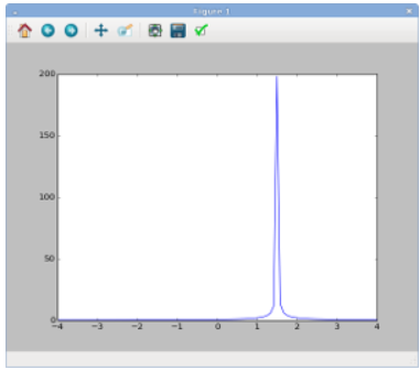
That's pretty much what we expect: the potential is peaked at \(X=1.5\), which is the position of the particle we specified in the program (via the variable named x0). The charge of the particle is given by the variable named q0, and we have assigned that the value \(1.0\). Hence, the potential is positive.

Now close the figure, and return to the Python command prompt. Note that Python is still running, even though your program has finished. From the command line, you can also examine the values of the variables which have been created by your program, simply by typing their names into the command prompt:

>>> x0
1.5
>>> phi
array([ 0.15384615    0.15432194    0.15480068    0.1552824  ....
          ....        0.28902404    0.28735963    0.28571429 ])

The value of x0 is a number, \(1.5\), which was assigned to it when our program ran. The value of phi is more complicated: it is an array, which is a special data structure containing a sequence of numbers. From the command line, you can inspect the individual elements of this array. For example, to see the value of the array's first element, type this:

>>> phi[0]
0.153846153846

As we've mentioned, index 0 refers to the first element of the array. This so-called zero-based indexing is a common practice in computing. Similarly, index 1 refers to the second element of the array, index 2 refers to the third element, etc.

You can also look at the length of the array, by calling the functionlen. This function accepts an array input and returns its length, as an integer.

>>> len(phi)
500

You can exit the Python command line at any time by typing Ctrl-d or exit().