1.3: Modularizing the Code

1.3.1: Designing a Potential Function

We could continue altering the above code in a straightforward way. For example, we could add more particles by adding variables x1, x2, q1, q2, and so forth, and altering our formula for computing phi. However, this is not very satisfactory: each time we want to consider a new collection of particle positions or charges, or change the number of particles, we would have to re-write the program's internal "logic"—i.e., the part that computes the potentials. In programming terminology, our program is insufficiently "modular". Ideally, we want to isolate the part of the program that computes the potential from the part that specifies the numerical inputs to the calculation, like the positions and charges.

To modularize the code, let's define a function that computes the potential of an arbitrary set of charged particles, sampled at an arbitrary set of positions. Such a function would need three sets of inputs:

• An array of particle positions \(\vec{x}\equiv [x_{0}, \cdots, x_{N-1}]\). (Don't get confused, by the way: we are using these \(N\) numbers to refer to the positions of \(N\) particles in a 1D space, not the position of a single particle in an \(N\)-dimensional space.)
• An array of particle charges \(\vec{q}\equiv [q_{0}, \cdots, q_{N-1}]\).
• An array of sampling points \(\vec{X}\equiv [X_{0}, \cdots, X_{M-1}]\), which are the points where we want to know \(\phi(X)\).

The number of particles, \(N\), and the number of sampling points, \(M\), should be arbitrary positive integers. Furthermore, \(N\) and \(M\) need not be equal.

The function we intend to write must compute the array

\[\begin{bmatrix}\phi(X_{0})\\ \phi(X_{1}) \\ \vdots \\ \phi(X_{M-1})\end{bmatrix}\]

which contains the value of the total electric potential at each of the sampling points. The total potential can be written as the sum of contributions from all particles. Let us define \(\phi_{j}(x)\) as the potential produced by particle \(j\):

\[\phi_{j(x)}\equiv\frac{q_{j}}{|x-x_{j}|}\]

Then the total potential is

\[\begin{bmatrix}\phi(X_0)\\ \phi(X_1) \\ \vdots \\ \phi(X_{M-1})\end{bmatrix} = \begin{bmatrix}\phi_0(X_0)\\ \phi_0(X_1) \\ \vdots \\ \phi_0(X_{M-1})\end{bmatrix} + \begin{bmatrix}\phi_1(X_0)\\ \phi_1(X_1) \\ \vdots \\ \phi_1(X_{M-1})\end{bmatrix} + \cdots + \begin{bmatrix}\phi_{N-1}(X_0)\\ \phi_{N-1}(X_1) \\ \vdots \\ \phi_{N-1}(X_{M-1})\end{bmatrix}.\]

1.3.2 Writing the Program

Let's code this up. Return to the file potentials.py, and delete the entire contents of the file. Then replace it with the following:

from scipy import *
import matplotlib.pyplot as plt

## Return the potential at measurement points X, due to particles
## at positions xc and charges qc.  xc, qc, and X must be 1D arrays,
## with xc and qc of equal length.  The return value is an array
## of the same length as X, containing the potentials at each X point.
def potential(xc, qc, X):
    M = len(X)
    N = len(xc)
    phi = zeros(M)
    for j in range(N):
        phi += qc[j] / abs(X - xc[j])
    return phi

charges_x  = array([0.2, -0.2])
charges_q  = array([1.5, -0.1])
xplot = linspace(-3, 3, 500)

phi = potential(charges_x, charges_q, xplot)

plt.plot(xplot, phi)
pmin, pmax = -50, 50
plt.ylim(pmin, pmax)
plt.show()

Figure \(\PageIndex{1}\)

When typing or pasting the above into your file, be sure to preserve the indentation (i.e., the number of spaces at the beginning of each line). Indentation is important in Python; as we'll see, it's used to determine program structure. Now save and run the program again:

• In the Windows GUI, type F5 in the editing window showing potentials.py.
• On GNU/Linux, type python -i potentials.py from the command line.
• Alternatively, from the Python command line, type import potentials, which will load and run your potentials.py file.

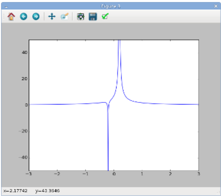
You should now see a figure like the one on the right, showing the electric potential produced by two particles, one at position \(x_{0}=0.2\) with charge \(q_{0}=1.5\) and the other at position \(x_{1}=-0.2\) with charge \(q_{1}=-0.1\).

There are less than \(20\) lines of actual code in the above program, but they do quite a lot of things. Let's go through them in turn:

Module Imports

The first two lines import the Scipy and Matplotlib modules, for use in our program. We have not yet explained how importing works, so let's do that now.

from scipy import *
import matplotlib.pyplot as plt

Each Python module, including Scipy and Matplotlib, defines a variety of functions and variables. If you use multiple modules, you might have a situation where, say, two different modules each define a function with the same name, but doing entirely different things. That would be Very Bad. To help avoid this, Python implements a concept called a namespace. Suppose you import a module (say Scipy) like this:

import scipy

One of the functions defined by Scipy is linspace, which we have already seen. This function was defined by the scipy module, and lies inside the scipy namespace. As a result, when you import the Scipy module using the import scipy line, you have to call the linspace function like this:

x = scipy.linspace(-3, 3, 500)

The scipy. in front says that you're referring to the linspace function that was defined in the scipy namespace. (Note: the online documentation for linspace refers to it as numpy.linspace, but the exact same function is also present in the scipy namespace. In fact, all numpy.* functions are replicated in the scipy namespace. So unless stated otherwise, we only have to import scipy.)

We will be using a lot of functions that are defined in the scipy namespace. Since it would be annoying to have to keep typing scipy. all over the place, we opt to use a slightly different import statement:

from scipy import *

This imports all the functions and variables in the scipy namespace directly into your program's namespace. Therefore, you can just call linspace, without the scipy. prefix. Obviously, you don't want to do this for every module you use, otherwise you'll end up with the name-clashing problem we alluded to earlier! The only module we'll use this shortcut with is scipy.

Another way to avoid having to type long prefixes is shown by this line:

import matplotlib.pyplot as plt

This imports the matplotlib.pyplot module (i.e., the pyplot module which is nested inside the matplotlib module). That's where plot, show, and other plotting functions are defined. The as plt in the above line says that we will refer to the matplotlib.pyplot namespace as the short form plt instead. Hence, instead of calling the plot function like this:

matplotlib.pyplot.plot(x, y)

we will call it like this:

plt.plot(x, y)

Comments

Let's return to the program we were looking at earlier. The next few lines, beginning with #, are "comments". Python ignores the # character and everything that follows it, up to the end of the line. Comments are very important, even in simple programs like this.

When you write your own programs, please remember to include comments. You don't need a comment for every line of code—that would be excessive—but at a minimum, each function should have a comment explaining what it does, and what the inputs and return values are.

Function Definition

Now we get to the function definition for the function named potential, which is the function that computes the potential:

def potential(xc, qc, X):
    M = len(X)
    N = len(xc)
    phi = zeros(M)
    for j in range(N):
        phi += qc[j] / abs(X - xc[j])
    return phi

The first line, beginning with def, is a function header. This function header states that the function is named potential, and that it has three inputs. In computing terminology, the inputs that a function accepts are called parameters. Here, the parameters are named xc, qc and X. As explained by the comments, we intend to use these for the positions of the particles, the charges of the particles, and the positions at which to measure the potential, respectively.

The function definition consists of the function header, together the rest of the indented lines below it. The function definition terminates once we get to a line which is at the same indentation level as the function header. (That terminating line is considered a separate line of code, which is not part of the function definition).

By convention, you should use 4 spaces per indentation level.

The indented lines below the function header are called the function body. This is the code that is run each time the function is called. In this case, the function body consists of six lines of code, which are intended to compute the total electric potential, according to the procedure that we have outlined in the preceding section:

• The first two lines define two helpful variables, M and N. Their values are set to the lengths of the X and xc arrays, respectively.
• The next line calls the zeros function. The input to zeros is M, the length of the X array (i.e., our function's third parameter). Therefore, zeros returns an array, of the same same length as X, with every element set to 0.0. For now, this represents the electric potential in the absence of any charges. We give this array the name phi.
• The function then iterates over each of the particles and add up its contribution to the potential, using a construct known as a for loop. The code for j in range(N): is the loop's "header line", and the next line, indented 4 spaces deeper than the header line, is the "body" of the loop.

  The header line states that we should run the loop body several times, with the variable j set to different values during each run. The values of j to loop over are given by range(N). This is a function call to the range function, with N (the number of electric charges) as the input. The range(N) function call returns a sequence specifying N successive integers, from 0 to N-1, inclusive. (Note that the last value in the sequence is N-1, not N. Because we start from 0, this means that there is a total of N integers in the sequence. Also, calling range(N) is the same as calling range(0,N).)

• For each j, we compute qc[j] / abs(X - xc[j]). This is an array whose elements are the values of the electric potential at the set of positions X, arising from the individual particle\(j\). In mathematical terms, we are calculating
  \[\phi_j(X) \equiv \frac{q_j}{|X - x_j|}\]

  using the array of positions X. We then add this array to phi. Once this is done for all j, the array phi will contain the desired total potential,
  \[\phi(X) = \sum_{j=0}^{N-1}\phi_j(X).\]

• Finally, we call return to specify the function's output, or return value. This is the array phi.

Top-Level Code: Numerical Constants

After the function definition comes the code to use the function:

charges_x  = array([0.2, -0.2])
charges_q  = array([1.5, -0.1])
xplot = linspace(-3, 3, 500)

Like the import statements at the beginning of the program, these lines of code lie at top level, i.e., they are not indented. The function header which defines the potential function is also at top level. Running a Python program consists of running its top level code, in sequence.

The above lines define variables to store some numerical constants. In the first two lines, charges_x and charges_q variables store the numerical values of the positions and charges we are interested in. These are initialized using the array function. You may be wondering why the array function call has square brackets nested in commas. We'll explain later, in part 2 of the tutorial.

On the third line, the linspace function call returns an array, whose contents are initialized to the 500 numbers between -3 and 3 (inclusive).

Next, we call the potential function, passing charges_x, charges_q and xplot as the inputs:

phi = potential(charges_x, charges_q, xplot)

These inputs provide the values of the function definition's parameters xc, qc, and X respectively. The return value of the function call is an array containing the total potential, evaluated at each of the positions specified in xplot. This return value is stored as the variable named phi.

Plotting

Finally, we create the plot:

plt.plot(xplot, phi)
pmin, pmax = -50, 50
plt.ylim(pmin, pmax)
plt.show()

We have already seen how the plot and show functions work. Here, prior to calling plt.show, we have added two extra lines to make the potential curve is more legible, by adjust the plot's y-axis bounds. The ylim function accepts two parameters, the lower and upper bounds of the y-axis. In this case, we set the bounds to -50 and 50 respectively. There is an xlim function to do the same for the x-axis.

Notice that in the line pmin, pmax = -50, 50, we set two variables (pmin and pmax) on the same line. This is a little "syntactic sugar" to make the code a little easier to read. It's equivalent to having two separate lines, like this:

pmin = -50
pmax = 50

We'll explain how this construct works in the next part of the tutorial.