5.1: The Basic Algorithm

Last updated
Save as PDF

Page ID: 34834

\( \newcommand{\vecs}[1]{\overset { \scriptstyle \rightharpoonup} {\mathbf{#1}} } \) \( \newcommand{\vecd}[1]{\overset{-\!-\!\rightharpoonup}{\vphantom{a}\smash {#1}}} \)\(\newcommand{\id}{\mathrm{id}}\) \( \newcommand{\Span}{\mathrm{span}}\) \( \newcommand{\kernel}{\mathrm{null}\,}\) \( \newcommand{\range}{\mathrm{range}\,}\) \( \newcommand{\RealPart}{\mathrm{Re}}\) \( \newcommand{\ImaginaryPart}{\mathrm{Im}}\) \( \newcommand{\Argument}{\mathrm{Arg}}\) \( \newcommand{\norm}[1]{\| #1 \|}\) \( \newcommand{\inner}[2]{\langle #1, #2 \rangle}\) \( \newcommand{\Span}{\mathrm{span}}\) \(\newcommand{\id}{\mathrm{id}}\) \( \newcommand{\Span}{\mathrm{span}}\) \( \newcommand{\kernel}{\mathrm{null}\,}\) \( \newcommand{\range}{\mathrm{range}\,}\) \( \newcommand{\RealPart}{\mathrm{Re}}\) \( \newcommand{\ImaginaryPart}{\mathrm{Im}}\) \( \newcommand{\Argument}{\mathrm{Arg}}\) \( \newcommand{\norm}[1]{\| #1 \|}\) \( \newcommand{\inner}[2]{\langle #1, #2 \rangle}\) \( \newcommand{\Span}{\mathrm{span}}\)

The best way to understand how Gaussian elimination works is to work through a concrete example. Consider the following \(N=3\) problem:

\[\begin{bmatrix}1 &2 &3 \\ 3 &2 &2 \\ 2 &6 &2\end{bmatrix} \begin{bmatrix} x_0 \\ x_1 \\ x_2 \end{bmatrix} = \begin{bmatrix}3 \\ 4 \\ 4\end{bmatrix}.\]

The Gaussian elimination algorithm consists of two distinct phases: row reduction and back-substitution.

5.1.1 Row Reduction

In the row reduction phase of the algorithm, we manipulate the matrix equation so that the matrix becomes upper triangular (i.e., all the entries below the diagonal are zero). To achieve this, we note that we can subtract one row from another row, without altering the solution. In fact, we can subtract any multiple of a row.

We will eliminate (zero out) the elements below the diagonal in a specific order: from top to bottom along each column, then from left to right for successive columns. For our \(3\times 3\) example, the elements that we intend to eliminate, and the order in which we will eliminate them, are indicated by the colored numbers \(0\), \(1\), and \(2\) in the following figure:

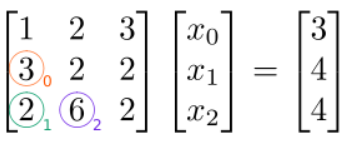
The first matrix element we want to eliminate is at \((1,0)\) (orange circle). To eliminate it, we subtract, from this row, a multiple of row \(0\). We will use a factor of \(3/1=3\):

\[(3x_0 + 2x_1 + 2x_2) - (3/1)(1x_0 + 2x_1 + 3x_2) = 4 - (3/1) 3\]

The factor of \(3\) we used is determined as follows: we divide the matrix element at \((1,0)\) (which is the one we intend to eliminate) by the element at \((0,0)\) (which is the one along the diagonal in the same column). As a result, the term proportional to \(x_{0}\) disappears, and we obtain the following modified linear equations, which possess the same solution:

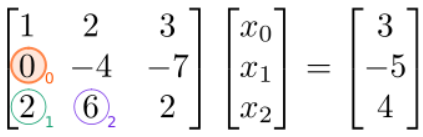
(Note that we have changed the entry in the vector on the right-hand side as well, not just the matrix on the left-hand side!) Next, we eliminate the element at \((2,0)\) (green circle). To do this, we subtract, from this row, a multiple of row \(0\). The factor to use is \(2/1=2\), which is the element at \((2,0)\) divided by the \((0,0)\) (diagonal) element:

\[(2x_0 + 6x_1 + 2x_2) - (2/1)(1x_0 + 2x_1 + 3x_2) = 4 - (2/1) 3\]

The result is

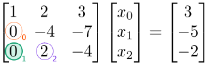
Next, we eliminate the \((2,1)\) element (blue circle). This element lies in column \(1\), so we eliminate it by subtracting a multiple of row \(1\). The factor to use is \(2/(-4)=-0.5\), which is the \((2,1)\) element divided by the \((1,1)\) (diagonal) element:

\[(0x_0 + 2x_1 - 4x_2) - (2/(-4))(0x_0 - 4x_1 - 7x_2) = -5 - (2/(-4)) (-2)\]

The result is

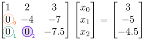
We have now completed the row reduction phase, since the matrix on the left-hand side is upper-triangular (i.e., all the entries below the diagonal have been set to zero).

5.1.2 Back-Substitution

In the back-substitution phase, we read off the solution from the bottom-most row to the top-most row. First, we examine the bottom row:

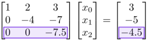
Thanks to row reduction, all the matrix elements on this row are zero except for the last one. Hence, we can read off the solution

\[x_{2}=(-4.5)/(-7.5)=0.6.\]

Next, we look at the row above:

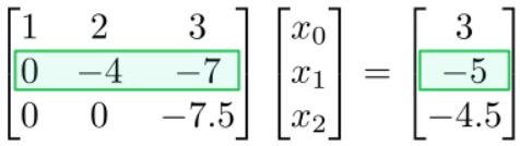
This is an equation involving \(x_{1}\) and \(x_{2}\). But from the previous back-substitution step, we know \(x_{2}\). Hence, we can solve for

\[x_1 = [-5 - (-7) (0.6)] / (-4) = 0.2.\]

Finally, we look at the row above:

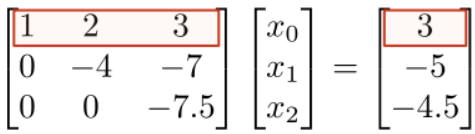
This involves all three variables \(x_{0}\), \(x_{1}\), and \(x_{2}\). But we already know \(x_{1}\) and \(x_{2}\), so we can read off the solution for \(x_{0}\). The final result is

\[\begin{bmatrix}x_0 \\ x_1 \\ x_2\end{bmatrix} = \begin{bmatrix}0.8 \\ 0.2 \\ 0.6\end{bmatrix}.\]

5.1.3 Runtime

Let's summarize the components of the Gaussian elimination algorithm, and analyze how many steps each part takes:

Row reduction
•	Step forwards through the rows. For each row \(n\),			\(N\) steps
	•	Perform pivoting (to be discussed below).		\(N-n +1 \sim N\) steps
	•	Step forwards through the rows larger than \(n\). For each such row \(m\),		\(N-n \sim N\) steps
		•	Subtract \((A'_{mn}/A'_{nn})\) times row \(n\) from the row \(m\) (where \(\mathbf{A}'\) is the current matrix). This eliminates the matrix element at \((m,n)\).	\(O(N)\) arithmetic operations
Back-substitution
•	Step backwards through the rows. For each row \(n\),			\(N\) steps
	•	Substitute in the solutions \(x_{m}\) for \(m>n\) (which are already found). Hence, find \(x_{n}\).		\(N-n \sim O(N)\) arithmetic operations

(The "pivoting" procedure hasn't been discussed yet; we'll do that in a later section.)

We conclude that the runtime of the row reduction phase scales as \(O(N^{3})\), and the runtime of the back-substitution phase scales as \(O(N^{2})\). The algorithm's overall runtime therefore scales as \(O(N^{3})\).