Heat Equation

In the Pendulum Experiment, we studied the Runge-Kutta algorithm for solving ordinary differential equations (ODEs). Here, we study techniques for solving partial differential equations (PDEs). The general problem of solving PDEs is huge; Press et al. in Numerical Recipes claim it requires an entire book.1 However, there are some simple cases. Separation of Variables: Consider the Schro¨dinger equation:

\[– \hbar^2/2m \frac{∂^2Ψ(x,t)}{∂x^2 } + V (x)Ψ(x,t) = i\hbar \frac{∂Ψ(x,t)}{∂t } \tag{1}\]

If we assume that the wave function can be written as a function of position times a function of time:

\[Ψ(x,t) = ψ(x)φ(t) \]

then:

\[\frac{1}{ψ(x)} [ –\hbar/2m \frac{∂^2Ψ(x)}{∂x^2 }+ V (x)ψ(x) ] = \frac{1}{\phi(t)} i\hbar \frac{d\phi}{dt } = c \tag{2}\]

where c is a constant. Thus we have turned the problem into two ordinary differential equations.

First order PDEs: If the equations are linear, then a closed solution can easily be found. If the equations are non-linear, a family of parametric solutions can be found. The standard Mathematica package Calculus‘PDSolve1‘ handles this latter case.

Second order PDEs: There are two general classes of these:

1. Poisson, sometimes called "elliptic." 1. § 17.0.

2. Cauchy, sometimes called "initial value." The Poisson equation is, of course:

\[\frac{∂^2u}{ ∂x^2} + \frac{∂^2u}{ ∂y^2} = ρ(x,t) \tag{3}\]

This type of equation turns out to be very easy to solve using a technique called a relaxation method. The Cauchy class of second order PDEs is subdivided further:

i. The wave equation (a hyperbolic form):

\[\frac{∂^2u}{ ∂t^2}= v^2 \frac{∂^2u}{ ∂x^2} \tag{4}\]

ii. The heat equation (a parabolic form):

\[\frac{∂u}{ ∂t} = \frac{∂}{ ∂x}( c \frac{∂u}{ ∂x}) \tag{5}\]

For both of these, you will discover that stability is a problem: many reasonable looking algorithms just don’t work unless care is taken.

In this Experiment, we will concentrate on the heat equation. Usually, u is the temperature. We will assume that we are solving the equation for a one dimensional slab of width L. We will usually assume that c is a constant so the heat equation becomes:

\[\frac{∂u(x,t)}{ ∂t} = c \frac{∂^2u(x,t)}{ ∂x^2}\]

We will adopt units where x/L → x and tc/L² → t, so the heat equation is now:

\[\frac{∂u(x,t)}{ ∂t} = \frac{∂^2u(x,t)}{ ∂x^2} \tag{6}\]

\[0 ≤ x ≤ 1\]

These notes are organized as follows:

I. Explicit algorithm.

II. Implicit algorithm.

III. Crank-Nicholson algorithm.

IV. Schro¨dinger’s equation.

V. References.

Note that the "usual" code listing is not included in this document. That is because you will be modifying some of the code to produce a new procedure, and cutting and pasting the code within the notebook is the simplest way to do this. Thus, the code listing appears in the notebook instead of these supplementary notes for the Experiment.

I. EXPLICIT ALGORITHM

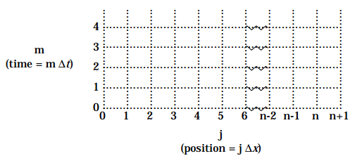
We imagine that we divide our one dimensional slab into n interior points, and will call the distance between each point ∆x. We will step through timesteps ∆t. We will be using the notation that:

\[u_j^m ≡ u(x_j = j\Delta x,t_m = m\Delta t) \tag{I.1}\]

\[0 ≤ j ≤ n+1 \]

\[(n + 1)∆x = 1\]

\[m = 0,1,2, ...\]

We will write the initial condition as:

\[u_j^0 = g (x) \tag{I.2}\]

and the boundary conditions as:

\[u_0^m = α \tag{I.3.a}\]

\[u_{n +1}^m = β \tag{I.3b}\]

It is reasonable to write the left hand side of the heat equation, Equation (6), as:

\[\frac{∂u}{∂t} = \frac{ u_j^{ m +1} – u_j^m}{\Delta t} \tag{I.4}\]

We write the right hand side of Equation (6) as:

\[\left.\frac{ ∂^2u}{∂x^2} \right|_{x_j} = (\left.\frac{∂x}{ ∂u} \right|_{x_j + \frac{1}{2}} – \left.\frac{ ∂u}{∂x} \right|_{x_j – \frac{1}{2}}) / \Delta x \tag{I.5}\]

Note that we write ∂u/∂x evaluated at two points that are not on our grid. This doesn’t matter because:

\[\left.\frac{∂x}{ ∂u} \right|_{x_j + \frac{1}{2} }= \frac{ u_{ j +1}^m – u_j^m}{\Delta x} \]

\[\left.\frac{∂x}{ ∂u} \right|_{x_j – \frac{1}{2}} = \frac{ u_{ j }^m – u_{j-1}^m}{\Delta x}\]

Thus, Equation (I.5) becomes:

\[\left.\frac{ ∂^2u(x,t)}{∂x^2} \right|_{x_j} = \frac{ 1}{\Delta x^2}(u_{j +1}^m –2u_j^m + u_{j –1}^m) \tag{I.6}\]

The above way of solving the second-order partial derivative is called the method of finite differences.

The heat equation states that Equation (I.4) equals Equation (I.6):

\[\frac{ u_j^{ m +1} – u_j^m}{\Delta t} = \frac{ 1}{\Delta x^2}(u_{j +1}^m –2u_j^m + u_{j –1}^m) \tag{I.7}\]

so:

\[u_j^{m +1} = u_j^m + \frac{ \Delta t}{\Delta x^2}(u_{j +1}^m –2u_j^m + u_{j –1}^m) \tag{I.8}\]

Note that the right hand side of Equation (I.8) contains values of u at time t_m = m∆t, and these terms are combined to give the value of u at the later time t_{m +1} = (m + 1)∆t. Once the values of u at time t_{m +1} = (m + 1)∆t are known we can then find the values at t_{m +2} = (m + 2)∆t, and so on. Thus we can solve the heat equation for all values of t using this explicit algorithm.

The determination of u_j ^{m +1} depends on knowing the values of u at three positions at the earlier time:

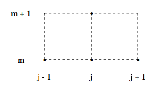
Note that this scheme does not allow one to determine u₀^{m +1} because we have no values for u_–1^m . But that does not matter: u₀^{m +1} is the value of u at the left side of the slab, and is given by the boundary condition Equation (I.3a). Similarly the boundary condition Equation (I.3b) gives the value for u_{n +1}^{m +1}. So Equation (I.8) is used only to evaluate the interior values of u^{m +1}.

The above way of solving the heat equation is pretty simple. Of the three algorithms you will investigate to solve the heat equation, this one is also the fastest and also can give the most accurate result. However, the result will be accurate only if you choose time steps ∆t and a space grid size ∆x such that:

\[\frac{ ∆t}{(∆x)^2} ≡µ≤ \frac{1}{2} \tag{I.9}\]

Solutions produced in violation of Equation (I.9) will be unstable, often producing ridiculous results. Note that this means that for a given time step ∆t the space grid size ∆x can not be too small. For a given space grid size, the time step can not be too big.

We will discuss later in this document the fact that even if the time step and space grid satisfy Equation (I.9), the explicit algorithm can still produce wrong results for some physical systems.

The reasons for the instability of the explicit algorithm is somewhat beyond the level of this course; consult the references for further information.2 However, we can justify Equation (I.9).

The heat equation also governs the diffusion of, say, a small quantity of perfume in the air. You probably already know that diffusion is a form of random walk so after a time t we expect the perfume has diffused a distance x ∝ √t. One solution to the heat equation gives the density of the gas as a function of position and time:

\[u (x,t) ≡ ρ(x,t) = \frac{e^{– \frac{x^2}{2σ^2 }}}{σ } \tag{I.10}\]

where:

\[σ=\sqrt{2ct}\]

and c is the heat constant defined in Equation (5), for which we usually have been choosing units so that it equals 1. In a diffusion context c is often called the diffusion constant. Equation (I.10) shows that the density of the diffusing gas is a Gaussian, and that the standard deviation describing the width of the Gaussian increases as the square root of t. This means that in a time ∆t, the molecules travel a distance ∆x on the order of:

\[\Delta x \approx \sqrt{2c\Delta t} = \sqrt{2\Delta t}\]

Thus, if we are solving the equations using an explicit algorithm, for a given ∆t:

\[\Delta x ≥ \sqrt{2\Delta t} \tag{I.11}\]

since otherwise the distribution is not spreading as fast as we know it should. A trivial rearrangement of Equation (I.11) gives:

\[\frac{\Delta t}{(\Delta x)^2} ≤ \frac{1}{2}\]

which is just Equation (I.9).

II. IMPLICIT ALGORITHM

Consider the following equation and compare it to Equation (I.7) from the previous section:

\[\frac{ u_j^{ m +1} – u_j^m}{\Delta t} = \frac{ 1}{(\Delta x)^2}(u_{j +1}^{m+1} –2u_j^{m+1} + u_{j –1}^{m+1}) \tag{II.1}\]

Here we are evaluating ∂2u/∂x 2 using finite differences at time t m +1 instead of t m. A moment’s reflection should convince you that Equation (II.1) is just as reasonable as Equation (I.7). We rearrange Equation (II.1):

\[(1+2µ)u_j^{m +1} – µ(u_{j +1}^{m+1} + u_{j -1}^{m+1} ) = u_j^m \tag{II.2}\]

where recall that:

\[µ = \frac{(\Delta x)^2}{ \Delta t}\]

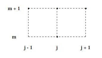
Thus we are trying to find u at times m+1 at three different positions j-1, j and j+1 from a single value of u at the earlier time m.

At first glance, this is impossible. However, consider an (n+2)×(n+2) identity matrix Id:

\[Id = \left(\begin{array}{ccc} 1&0&0&.&0 \\ 0&1&0&.&0 \\ 0&0&1&.&0 \\ .&.&.&.&. \\0&0&0&.&1 \end{array} \right)\]

an (n+2)×(n+2) (2,-1) triangular matrix A:

\[A = \left(\begin{array}{ccc} 2&-1&0&.&0&0 \\ -1&2&-1&.&0&0 \\ 0&-1&2&.&0&0 \\ .&.&.&.&.&. \\ 0&0&0&.&2&-1\\ 0&0&0&.&-1&2 \end{array} \right)\]

and an n+2 dimensional column matrix b → : -

\[\overrightarrow{b} =\left(\begin{array}{ccc} µα \\ 0\\ 0 \\ .\\ µβ \end{array} \right)\]

Then the entire set of equations for all values of j given by Equation (II.2) can be written as:

\[(Id + µA) \overrightarrow{u}^{m +1} = \overrightarrow{u}^{m} + \overrightarrow{b} \tag{II.3}\]

where:

\[\overrightarrow{u} = \left(\begin{array}{ccc} u_0 \\ u_1\\ u_2 \\ .\\ u_n \\ u_{n +1} \end{array} \right) . \]

If we know →u m, the values of u at time m, Equation (II.3) may be solved for →u m +1 using, for example, the LU decomposition that you studied in the Exercise.

The above technique for solving the heat equation is called an implicit algorithm. You will discover in the Experiment that this algorithm is stable for all values of µ. That is the good news. There is also some bad news: the implicit technique is much slower than the explicit one and is also much less accurate for a given value of timestep ∆t and space grid size ∆x.

III. CRANK-NICHOLSON ALGORITHM

The explicit algorithm begins with:

\[\frac{ u_m^{ m +1} – u_j^m}{\Delta t} = \frac{ 1}{(\Delta x)^2}(u_{j +1}^m –2u_j^m + u_{j –1}^m)\]

while the implicit one begins with:

\[\frac{ u_m^{ m +1} – u_j^m}{\Delta t} = \frac{ 1}{(\Delta x)^2}(u_{j +1}^{m+1} –2u_j^{m+1} + u_{j –1}^{m+1})\]

Average these two equations:

\[\frac{ u_m^{ m +1} – u_j^m}{\Delta t} = \frac{ 1}{(2} \frac{ 1}{(\Delta x)^2} (u_{j +1}^m –2u_j^m + u_{j –1}^m+u_{j +1}^{m+1} –2u_j^{m+1} + u_{j –1}^{m+1}) \tag{III.1}\]

In terms of the matrices defined in the previous section, we can write Equation (III.1) as:

\[(Id + \frac{µ}{2}A) \overrightarrow{u}^{m +1} =(Id - \frac{µ}{2}A) \overrightarrow{u}^{m} + \overrightarrow{b} \tag{III.2}\]

This equation is, of course, solvable using LU decomposition. We are finding the values of uj –1 m +1, uj m +1 and uj +1 m +1 from the values of uj –1 m , uj m and uj +1 m .

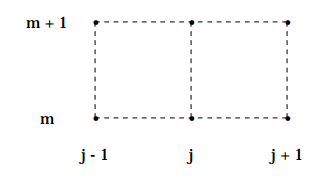
The above is the Crank-Nicholson algorithm. You will discover that it maintains the absolute stability of the implicit algorithm while recovering some of the accuracy of the explicit one.

IV. SCHRO¨ DINGER’S EQUATION

Assuming h⁄ = 1 and m = 1/2, Schro¨dinger’s equation is:

\[i \frac{ ∂Ψ(x,t)}{∂t} = HΨ(x,t) \tag{IV.1}\]

\[H = \frac{ ∂^2}{– ∂x^2} + V (x)\]

In the late 1960’s, Goldberg, Schey and Schwartz had a good idea for a lecture demonstration in quantum mechanics.3 They decided to solve this equation using thennew computer technology to produce a movie. The initial conditions for Equation (IV.1) are

_{3. Goldberg, Schey and Schwartz, Amer. Jour. Phys. 35, (1967) 177.}

\[Ψ(x, 0) = g (x)\]

and the boundary conditions are:

\[Ψ(\infty,t) = Ψ(–\infty,t) = 0\]

The solution to Equation (IV.1) can be written as:

\[Ψ(x,t) = e^{ –iHt}Ψ(x, 0) \tag{IV.2}\]

Expand Equation (IV.2) and throw out higher order terms:

\[Ψ(x,t + \Delta t) \approx (1 – iHt)Ψ(x,t)\tag{IV.3}\]

Thus if we know Ψ(x,t) we can produce a time series of values for Ψ at times t + ∆t, t + 2∆t, ... . Using finite differences to evaluate the ∂2/∂x 2 term in the Hamiltonian H, the right hand side of Equation (IV.3) will give a term involving (Ψj –1 m – 2Ψj m + Ψj +1 m ). This should be recognisable to you as an explicit algorithm. We can multiply Equation (IV.2) by e iHt and expand to get:

\[(1 + iHT)Ψ(x,t + \Delta t) \approx Ψ(x,t) \tag{IV.4}\]

Now evaluating the Hamiltonian using finite differences will give a term involving (Ψj –1 m +1 – 2Ψj m +1 + Ψj +1 m +1) on the left hand side. This is, of course, just an implicit algorithm. Everything we have said about explicit and implicit algorithms applies to these cases too. However, the physics of Quantum Mechanics puts an additional constraint on Ψ:

\[ ∫ _{x=–∞}^∞ Ψ*(x,t)Ψ(x,t)dx = 1 \tag{IV.5}\]

for all times t. This is called unitarity and physically means that the probability that the object being described by the wave function is somewhere between x = –∞ and x = ∞ is one.

It has been known since long before the invention of the computer that Equations (IV.3) and (IV.4) violate unitarity. This means that neither the explicit or implicit algorithm can be used to solve Schro¨dinger’s equation because they both violate a physical principle.

A long-known equation that does not violate unitarity is called Cayley’s form. Multiply Equation (IV.2) by e iHt/2 and expand both sides:

\[(1 + \frac{ i}{2} Ht)Ψ(x,t + \Delta t) = (1 – \frac{ i}{2} Ht)Ψ(x,t) \tag{IV.6}\]

Using finite differences to evaluate the ∂2/∂x 2 terms in the Hamiltonian on both sides of the equation will give us a Crank-Nicholson algorithm.

The lesson to be learned here is that just knowing the numerical methods is sometimes not sufficient. Just as for the pendulum, where the physics pointed us to the symplectic algorithm, here the physics points us to a Crank-Nicholson algorithm when solving Schro¨dinger’s equation.

V. REFERENCES

• Gene H. Golub and James M. Ortega, Scientific Computing and Differential Equations (Academic Press, 1992), Chapter 7.

• William H. Press, Brian P. Flannery, Saul A. Teukolsky, and William T. Vetterling, Numerical Recipes: The Art of Scientific Computing or Numerical Recipes in C: The Art of Scientific Computing (Cambridge Univ. Press), Chapter 17.

Examples of solving Poisson’s equation using relaxation methods, and a visualisation of Schro¨dinger’s equation solved using a Crank-Nicholson algorithm may be found at: emerald.math.buffalo.edu/˜ringland/instruction/pde/