3.1: Minkowski Metric
( \newcommand{\kernel}{\mathrm{null}\,}\)
Two observers both measure the time separation and spatial separation of two explosions that occur in interstellar space. One observer finds the explosions to be separated by 22s and 5.5×10⁹m.
- Is it possible that the other observer detects the two explosions as simultaneous? If so, how far apart are the events in this second frame?
- Is it possible that the other observer detects the two explosions as occurring at the same point? If so, how far apart in time are the two explosions in this second frame?
In classical three-dimensional space, the distance between two events can be determined by Pythagoras’ Theorem,
(dr)2=(dx)2+(dy)2+(dz)3
This distance is the same for any two observers, even if their individual measurements of x−, y−, and z-separation are different. This relationship forms a method of calculating distance in three-dimensional space and is referred to as the metric of three-dimensional flat space.
In Special Relativity, Pythagoras’ Theorem is not a valid way to calculate the distance between two events. Hermann Minkowski discovered that if the temporal (dt) and spatial (dx, dy, dz) separation between two events are combined in the following way,
(ds)2=(cdt)2−((dx)2+(dy)2+(dz)3)
the resulting quantity, the spacetime interval, is the same for all observers. This result is the metric of the four-dimensional flat spacetime that obeys Special Relativity. This metric is referred to as the Minkowski metric.
Since this combination of spatial and temporal separations is the same for all observers, we can use it to answer the above question. Label the two observers #1 and #2, and, if the events are simultaneous for observer #2, dt2=0.
Since the distance between events in frame #2 cannot be the square-root of a negative number, it is impossible for any other observer to see these two events as simultaneous.
For part b, if the two events are to be located at the same point,
Therefore, it is possible that another observer can see the two explosions as occurring at exactly the same point in space, separated by 12.2 s of time.
Solving Relativity Problems Geometrically
Particle accelerators routinely accelerate particles to close to the speed of light. Imagine an electron traveling at 0.9995c in a linear accelerator of length 3.2 km. How long does it take the electron to travel the length of the accelerator, as measured by the electron?
First, find the time in the laboratory frame using basic kinematics:
t=Δxv=3200m0.9995c=1.07×10⁻⁵s
This problem could now be easily solved using the time dilation relationship from special relativity. However, it can also be solved by a purely geometrical approach using the Minkowski metric.
With observer #1 the laboratory and #2 the electron, and the two events the electron beginning its journey and ending its journey (which both occur at the same point in the electron’s frame),
The Minkowski metric automatically incorporates all of the relationships we discussed while studying special relativity. Those relationships are properties of spacetime, not really relationships between objects occupying spacetime, and are thus built into the basic metric of spacetime. This view of examining the metric of spacetime to determine what happens to objects in spacetime forms the conceptual framework of general relativity.
Minkowski Metric in Polar Coordinates
We are free to express the Minkowski metric in whatever coordinate system is most useful for the problem under investigation. For example, the metric expressed in polar coordinates is:
(ds)2=(cdt)2−(dr)2−r2(dϕ)2
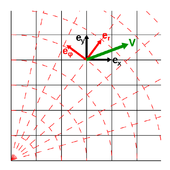
Notice (in Figure 3.1.1) that each small “step” in the radial direction, dr, is exactly the same length. The metric reflects this fact because there is no multiplicative factor in front of the dr term.

Figure 3.1.1: Transformation to polar coordinates, showing unit basis vectors. (CC BY-SA; Maksim).
However, the length of a “step” in the tangential direction, dϕ, depends on how far you are from the origin. The farther you are from the origin, the longer a single step in dϕ is. This is reflected by the multiplicative factor of ‘r’ in the tangential part of the metric. (As r gets big, a single step in dϕ gets big.)
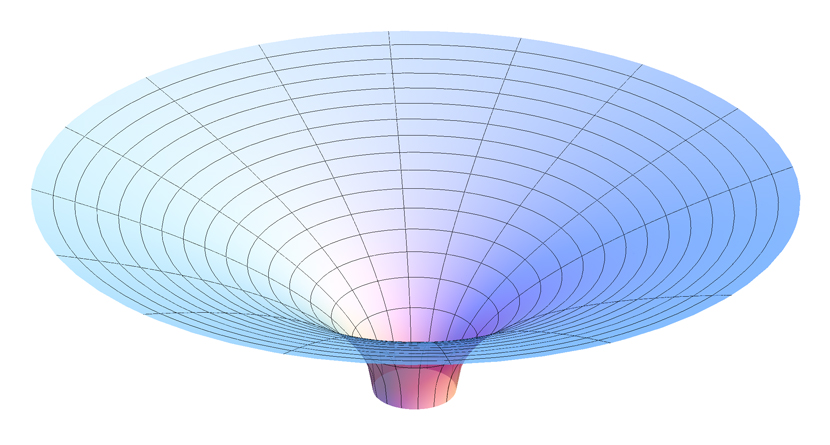
What would it mean if there were similar multiplicative factors in front of the temporal and radial parts of the metric? A factor in front of the dt part of the metric would mean that steps in dt (i.e., clicks of a clock) would be of different duration in different places. A factor in front of the radial part would mean that radial steps were of different lengths in different places. It would be like taking the coordinate grid shown above and stretching it by different amounts in different places, resulting in a coordinate system (and underlying space that the coordinate system is trying to represent) that is no longer flat, but rather warped or curved (Figure 3.1.2).

Figure 3.1.2: (CC BY-SA; )
For example, if the radial part of the metric was multiplied by a factor that got large as r got small, this would result in a coordinate system that looked something like the one in Figure 3.1.2. Notice that the radial steps get larger and larger as the radial distance gets smaller and smaller. Also notice that there is really no way to adequately draw this coordinate system on a flat surface; the coordinate system is intrinsically curved.


