
2.2: States, Observables and Eigenvalues


- Last updated
- Mar 4, 2022
- Save as PDF

( \newcommand{\kernel}{\mathrm{null}\,}\)
From the first postulate we see that the state of a quantum system is given by the state vector |ψ(t)⟩ (or the wavefunction ψ(→x,t)). The state vector contains all possible information about the system. The state vector is a vector in the Hilbert space. A Hilbert space H is a complex vector space that possess an inner product.
An example of Hilbert space is the usual Euclidean space of geometric vectors. This is a particularly simple case since the space in this case is real. In general as we will see, Hilbert space vectors can be complex (that is, some of their components can be complex numbers). In the 3D Euclidean space we can define vectors, with a representation such as →v={vx,vy,vz} or :
→v=[vxvyvz]
This representation corresponds to choose a particular basis for the vector (in this case, the usual {x,y,z} coordinates). We can also define the inner product between two vectors, →v and →u (which is just the usual scalar product):
→v⋅→u=[vxvyvz]⋅[uxuyuz]=vxux+vyux+vzuz
Notice that we have taken the transpose of the vector →v,→vT in order to calculate the inner product. In general, in a Hilbert space, we can define the dual of any vector. The Dirac notation makes this more clear.
The notation |ψ⟩ is called the Dirac notation and the symbol |⋅⟩ is called ket. This is useful in calculating inner products of state vectors using the bra ⟨⋅| which is the dual of the ket), for example ⟨φ|. An inner product is then written as ⟨φ∣ψ⟩ (this is a bracket, hence the names).
We will often describe states by their wavefunction instead of state vector. The wavefunction is just a particular way of writing down the state vector, where we express the state vector in a basis linked to the position of a particle itself (this is called the position representation). This particular case is however the one we are mostly interested in this course. Mathematically, the wavefunction is a complex function of space and time. In the position representation (that is, the position basis) the state is expressed by the wavefunction via the inner product ψ(x)=⟨x∣ψ⟩.
The properties of Hilbert spaces, kets and bras and of the wavefunction can be expressed in a more rigorous mathematical way. In this course as said we are mostly interested in systems that are nicely described by the wavefunction. Thus we will just use this mathematical tool, without delving into the mathematical details. We will see some more properties of the wavefunction once we have defined observables and measurement.
All physical observables (defined by the prescription of experiment or measurement ) are represented by a linear operator that operates in the Hilbert space H (a linear, complex, inner product vector space).
In mathematics, an operator is a type of function that acts on functions to produce other functions. Formally, an operator is a mapping between two function spaces2 A : g(I)→f(I) that assigns to each function g∈g(I) a function f=A(g)∈f(I).
Examples of observables are what we already mentioned, e.g. position, momentum, energy, angular momentum. These operators are associated to classical variables. To distinguish them from their classical variable counterpart, we will thus put a hat on the operator name. For example, the position operators will be ˆx,ˆy,ˆz. The momentum operators ˆpx,ˆpy,ˆpz and the angular momentum operators ˆLx,ˆLy,ˆLz. The energy operator is called Hamiltonian (this is also true in classical mechanics) and is usually denoted by the symbol H.
There are also some operators that do not have a classical counterpart (remember that quantum-mechanics is more general than classical mechanics). This is the case of the spin operator, an observable that is associated to each particle (electron, nucleon, atom etc.). For example, the spin of an electron is usually denoted by S; this is also a vector variable (i.e. we can define \(S_{x}, S_{y}, S_{z})). I am omitting here the hat since there is no classical variable we can confuse the spin with. While the position, momentum etc. observable are continuous operator, the spin is a discrete operator.
The second postulate states that the possible values of the physical properties are given by the eigenvalues of the operators.
2 A function space f(I) is a collection of functions satisfying certain properties.
Eigenvalues and eigenfunctions of an operator are defined as the solutions of the eigenvalue problem:
A[un(→x)]=anun(→x)
where n = 1, 2, . . . indexes the possible solutions. The an are the eigenvalues of A (they are scalars) and un(→x) are the eigenfunctions.
The eigenvalue problem consists in finding the functions such that when the operator A is applied to them, the result is the function itself multiplied by a scalar. (Notice that we indicate the action of an operator on a function by A[f(⋅)]).
You should have seen the eigenvalue problem in linear algebra, where you studied eigenvectors and eigenvalues of matrices. Consider for example the spin operator for the electron S. The spin operator can be represented by the following matrices (this is called a matrix representation of the operator; it’s not unique and depends on the basis chosen):
Sx=12(0110),Sy=12(0−ii0),Sz=12(100−1)
We can calculate what are the eigenvalues and eigenvectors of this operators with some simple algebra. In class we considered the eigenvalue equations for Sx and Sz. The eigenvalue problem can be solved by setting the determinant of the matrix Sα−s1 equal to zero. We find that the eigenvalues are ±12 for both operators. The eigenvectors are different:
vz1=[10],vz2=[01]
vx1=1√2[11],vx2=1√2[1−1]
We proved also that v1⋅v2=0 (that is, the eigenvectors are orthogonal) and that they form a complete basis (we can write any other vector, describing the state of the electron spin, as a linear combination of either the eigenvectors of Sz or of Sx).
The eigenvalue problem can be solved in a similar way for continuous operators. Consider for example the differential operator, d[⋅]dx. The eigenvalue equation for this operator reads:
df(x)dx=af(x)
where a is the eigenvalue and f(x) is the eigenfunction.
Question
what is f(x)? What are all the possible eigenvalues (and their corresponding eigenfunctions)?
The eigenvalue equation for the operator is xd[⋅]dx is:
xdf(x)dx=af(x)
which is solved by f(x)=xn, a = n.
The ”standard” Gaussian function 1√2πe−x2/2 is the eigenfunction of the Fourier transform. The Fourier transform is an operation that transforms one complex-valued function of a real variable into another one (thus it is an operator):
Fx:f(x)→˜f(k), with ˜f(k)=Fx[f(x)](k)=1√2π∫∞−∞f(x)e−ikxdx
Notice that sometimes different normalizations are used. With this definition, we also find that the inverse Fourier transform is given by:
F−1k:˜f(k)→f(x),f(x)=1√2π∫∞−∞˜f(k)eikxdk
Let’s now turn to quantum mechanical operators.
The position operator for a single particle ˆ→x is simply given by the scalar →x. This means that the operator ˆ→x acting on the wavefunction ψ(→x) simply multiplies the wavefunction by →x. We can write
ˆ→x[ψ(→x)]=→xψ(→x).
We can now consider the eigenvalue problem for the position operator. For example, for the x-component of →x this is written as:
ˆx[un(x)]=xnun(x)→xun(x)=xnun(x)
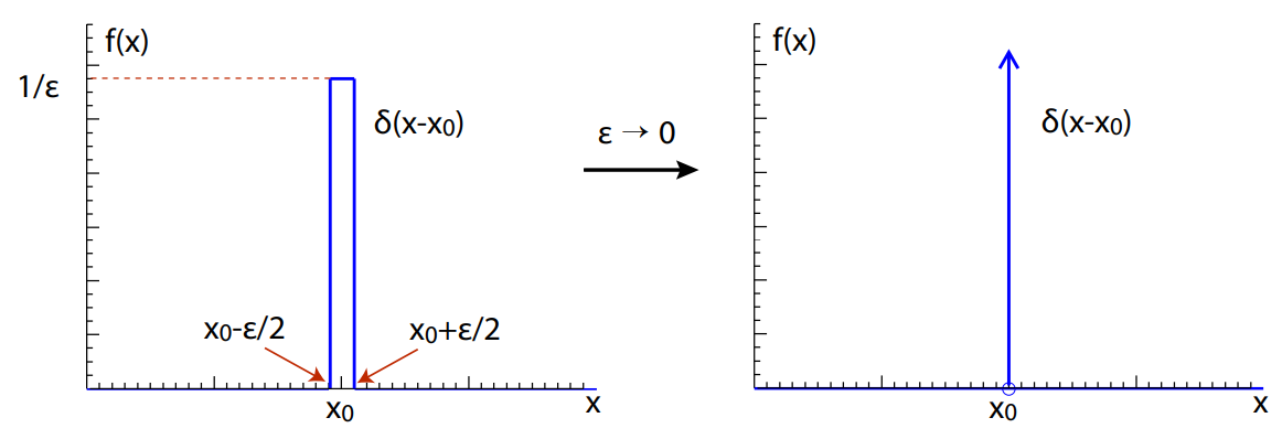
where we used the definition of the position operator. Here xn is the eigenvalue and un(x) the eigenfunction. The solution to this equation is not a proper function, but a distribution (a generalized function): the Dirac delta function: un(x)=δ(x−xn)
Dirac Delta function δ(x−x0) is equal to zero everywhere except at x0 where it is infinite. The Dirac Delta function also has the property that ∫∞−∞δ(x)dx=1 and of course xδ(x−x0)=x0δ(x−x0) (which corresponds to the eigenvalue problem above). We also have:
∫dxδ(x−x0)f(x)=f(x0)
That is, the integral of any function multiplied by the delta function gives back the function itself evaluated at the point x0. [See any textbook (and recitations) for other properties.]
How many solutions are there to the eigenvalue problem defined above for the position operator? One per each possible position, that is an infinite number of solutions. Conversely, all possible positions are allowed values for the measurement of the position (a continuum of solutions in this case).
The momentum operator is defined (in analogy with classical mechanics) as the generator of translations. This means that the momentum modifies the position of a particle from →x to →x+d→x. It is possible to show that this definition gives the following form of the position operator (in the position representation, or position basis)
ˆpx=−iℏ∂∂x,ˆpy=−iℏ∂∂y,ˆpz=−iℏ∂∂z
or in vector notation ˆp=−iℏ∇. Here ℏ is the reduced Planck constant h/2π (with h the Planck constant) with value
ℏ=1.054×10⁻³⁴ J s.
Planck’s constant is introduced in order to make the values of quantum observables consistent with the corresponding classical values.
We now study the momentum operator eigenvalue problem in 1D. The problem’s statement is
ˆpx[un(x)]=pnun(x)→−iℏ∂un(x)∂x=pnun(x)
This is a differential equation that we can solve quite easily. We set k=p/ℏ and call k the wavenumber (for reasons clear in a moment). The differential equation is then
∂un(x)∂x=iknun(x)
which has as solution the complex function:
un(x)=Aeiknx=Aeipnhx
The momentum eigenfunctions and eigenvalues are thus un=Aeiknx and kn.
Now remember the meaning of the eigenvalues. By the second postulate, the eigenvalues of an operator are the possible values that one can obtain in a measurement.
Obs. 1 There are no restrictions on the possible values obtained from a momentum measurements. All values p=ℏk are possible.
Obs. 2 The eigenfunction un(x) corresponds to a wave traveling to the right with momentum pn=ℏkn. This was also expressed by De Broglie when he postulated the existence of matter waves.
Louis de Broglie (1892-1987) was a French physicist. In his Ph.D thesis he postulated a relationship between the momentum of a particle and the wavelength of the wave associated with the particle (1922). In de Broglie’s equation a particle wavelength is the Planck’s constant divided by the particle momentum. We can see this behavior in the electron interferometer video3. For classical objects the momentum is very large (since the mass is large), then the wavelength is very small and the object loose its wave behavior. De Broglie equation was experimentally confirmed in 1927 when physicists Lester Germer and Clinton Davisson fired electrons at a crystalline nickel target and the resulting diffraction pattern was found to match the predicted values.
3 A. Tonomura, J. Endo, T. Matsuda, T. Kawasaki and H. Ezawa, Am. J. of Phys. 57, 117 (1989)
Properties of eigenfunctions
From these examples we can notice two properties of eigenfunctions which are valid for any operator:
- The eigenfunctions of an operator are orthogonal functions. We will as well assume that they are normalized. Consider two eigenfunctions un,um of an operator A and the inner product defined by ⟨f∣g⟩=∫d3xf∗(x)g(x). Then we have
∫d3xu∗m(x)un(x)=δnm - The set of eigenfunctions forms a complete basis.
This means that any other function can be written in terms of the set of eigenfunctions {un(x)} of an operator A:
f(x)=∑ncnun(x), with cn=∫d3xu∗n(x)f(x)
[Note that the last equality is valid iif the eigenfunctions are normalized, which is exactly the reason for normalizing them].
If the eigenvalues are a continuous parameter, we have a continuum of eigenfunctions, and we will have to replace the sum over n with an integral.
Consider the two examples we saw. From the property of the Dirac Delta function we know that we can write any function as:
f(x)=∫dx′δ(x′−x)f(x′)
We can interpret this equation as to say that any function can be written in terms of the position eigenfunction δ(x′−x) (notice that we are in the continuous case mentioned before, since the x-eigenvalue is a continuous function). In this case the coefficient cn becomes also a continuous function
cn→c(xn)=∫dxδ(x−xn)f(x)=f(xn).
This is not surprising as we are already expressing everything in the position basis.
If we want instead to express the function f(x) using the basis given by the momentum operator eigenfunctions we have: (consider 1D case)
f(x)=∫dkuk(x)c(k)=∫dkeikxc(k)
where again we need an integral since there is a continuum of possible eigenvalues. The coefficient c(k) can be calculated from
c(k)=∫dxu∗k(x)f(x)=∫dxe−ikxf(x)
We then have that c(k) is just the Fourier transform of the function f(x) (up to a multiplier).
The Fourier transform is an operation that transforms one complex-valued function of a real variable into another:
Fx:f(x)→˜f(k), with ˜f(k)=Fx[f(x)](k)=1√2π∫∞−∞f(x)e−ikxdx
Notice that sometimes different normalizations are used. With this definition, we also find that the inverse Fourier transform is given by:
F−1k:˜f(k)→f(x),f(x)=1√2π∫∞−∞˜f(k)eikxdk
Review of linear Algebra
This is a very concise review of concepts in linear algebra, reintroducing some of the ideas we saw in the previous paragraphs in a slightly more formal way.
Vectors and vector spaces
Quantum mechanics is a linear theory, thus it is well described by vectors and vector spaces. Vectors are mathematical objects (distinct from scalars) that can be added one to another and multiplied by a scalar. In QM we denote vectors by the Dirac notation: |ψ⟩,|φ⟩,…. Then, these have the properties:
- If |ψ1⟩ and |ψ2⟩ are vectors, then |ψ3⟩=|ψ1⟩+|ψ2⟩ is also a vector.
- Given a scalar s, |ψ4⟩=s|ψ1⟩ is also a vector.
A vector space is a collection of vectors. For example, for vectors of finite dimensions, we can define a vector space of dimensions N over the complex numbers as the collection of all complex-valued N-dimensional vectors.
A familiar example of vectors and vector space are the Euclidean vectors and the real 3D space.
Another example of a vector space is the space of polynomials of order n. Its elements, the polynomials Pn=a0+a1x+a2x2+⋯+anxn can be proved to be vectors since they can be summed to obtain another polynomial and multiplied by a scalar. The dimension of this vector space is n + 1.
In general, functions can be considered vectors of a vector space with infinite dimension (of course, if we restrict the set of functions that belong to a given space, we must ensure that this is still a well-defined vector space. For example, the collection of all function f(x) bounded by 3[f(x)<3,∀x] is not a well defined vector-space, since sf(x) (with s a scalar > 1) is not a vector in the space.
Inner product
We denote by ⟨ψ∣φ⟩ the scalar product between the two vectors |ψ⟩ and |φ⟩. The inner product or scalar product is a mapping from two vectors to a complex scalar, with the following properties:
- It is linear in the second argument: ⟨ψ∣a1φ1+a2φ2⟩=a1⟨ψ∣φ1⟩+a2⟨ψ∣φ2⟩.
- It has the property of complex conjugation: ⟨ψ∣φ⟩=⟨φ∣ψ⟩∗.
- It is positive-definite: ⟨ψ∣ψ⟩=0⇔|ψ⟩=0.
For Euclidean vectors the inner product is the usual scalar product →v1⋅→v2=|→v1||→v2|cosϑ.
For functions, the inner product is defined as:
⟨f∣g⟩=∫∞−∞f(x)∗g(x)dx
Linearly independent vectors (and functions)
We can define linear combinations of vectors as |ψ⟩=a1|φ1⟩+a2|φ2⟩+…. If a vector cannot be expressed as a linear superposition of a set of vectors, than it is said to be linearly independent from these vectors. In mathematical terms, if
|ξ⟩≠∑iai|φi⟩,∀ai
then |ξ⟩ is linearly independent of the vectors {|φi⟩}.
Basis
A basis is a linearly independent set of vectors that spans the space. The number of vectors in the basis is the vector space dimension. Any other vector can be expressed as a linear combination of the basis vectors. The basis is not unique, and we will usually choose an orthonormal basis.
For the Polynomial vector space, a basis are the monomials {xk},k=0,…,n. For Euclidean vectors the vectors along the 3 coordinate axes form a basis.
We have seen in class that eigenvectors of operators form a basis.
Unitary and Hermitian operators
An important class of operators are self adjoint or Hermitian operators, as observables are described by them. We need first to define the adjoint of an operator A. This is denoted A† and it is defined by the relation:
⟨(A†ψ)∣φ⟩=⟨ϕ∣(Aψ)⟩∀{|ψ⟩,|φ⟩}
This condition can also be written (by using the second property of the inner product) as:
⟨ψ|A†|φ⟩=⟨φ|A|ψ⟩∗
If the operator is represented by a matrix, the adjoint of an operator is the conjugate transpose of that operator: A†k,j=⟨k|A†|j⟩=⟨j|A|k⟩∗=A∗j,k.
A self adjoint operator is an operator such that A† = A, or more precisely
⟨ψ|A|φ⟩=⟨φ|A|ψ⟩∗
For matrix operators, Aki=A∗ik.
An important properties of Hermitian operators is that their eigenvalues are always real (even if the operators are defined on the complex numbers). Then, all the observables must be represented by hermitian operators, since we want their eigenvalues to be real, as the eigenvalues are nothing else than possible outcomes of experiments (and we wouldn’t want the position of a particle, for example, to be a complex number).
Then, for example, the Hamiltonian of any system is an hermitian operator. For a particle in a potential, it’s easy to check that the operator is real, thus it is also hermitian.
U are such that their inverse is equal to their adjoint: U−1=U†, or
UU†=U†U=1.
We will see that the evolution of a system is given by a unitary operator, which implies that the evolution is time-reversible.