
9.5: The Klien-Gordon and Relativistic Schrödinger Equations


- Last updated
- Jan 29, 2022
- Save as PDF

( \newcommand{\kernel}{\mathrm{null}\,}\)
Now let me switch gears and discuss the basics of relativistic quantum mechanics of particles with a non-zero rest mass m. In the ultra-relativistic limit pc≫mc2 the quantization scheme of such particles may be essentially the same as for electromagnetic waves, but for the intermediate energy range, pc∼mc2, a more general approach is necessary. Historically, the first attempts 47 to extend the non-relativistic wave mechanics into the relativistic energy range were based on performing the same transitions from classical observables to their quantum-mechanical operators as in the non-relativistic limit: p→ˆp=−iℏ∇,E→ˆH=iℏ∂∂t. The substitution of these operators, acting on the Schrödinger-picture wavefunction Ψ(r,t), into the classical relation (1) between the energy E and momentum p (for of a free particle) leads to the following formulas:
| Non-relativistic limit | Relativistic case | |
|---|---|---|
| Classical mechanics | E=12mp2 | E2=c2p2+(mc2)2 |
| Wave mechanics | iℏ∂∂tΨ=12m(−iℏ∇)2Ψ | (iℏ∂∂t)2Ψ=c2(−iℏ∇)2Ψ+(mc2)2Ψ |
The resulting equation for the non-relativistic limit, in the left-bottom cell of the table, is just the usual Schrödinger equation (1.28) for a free particle. Its relativistic generalization, in the right-bottom cell, usually rewritten as (1c2∂2∂t2−∇2)Ψ+μ2Ψ=0, with μ≡mcℏ is called the Klein-Gordon (or sometimes "Klein-Gordon-Fock") equation. The fundamental solutions of this equation are the same plane, monochromatic waves Ψ(r,t)∝exp{i(k⋅r−ωt)}. as in the non-relativistic case. Indeed, such waves are eigenstates of the operators (83), with eigenvalues, respectively, p=ℏk, and E=ℏω, so that their substitution into Eq. (84) immediately returns us to Eq. (1) with the replacements (86): E±=ℏω±=±[(ℏck)2+(mc2)2]1/2. Though one may say that this dispersion relation is just a simple combination of the classical relation (1) and the same basic quantum-mechanical relations (86) as in non-relativistic limit, it attracts our attention to the fact that the energy ℏω as a function of the momentum ℏk has two branches, with E (p) =−E+(p)− see Fig. 6a. Historically, this fact has played a very important role in spurring the fundamental idea of particle-antiparticle pairs. In this idea (very similar to the concept of electrons and holes in semiconductors, which was discussed in Sec. 2.8), what we call the "vacuum" actually corresponds to all quantum states of the lower branch, with energies E−(p)<0, being completely filled, while the states on the upper branch, with energies E+(p)>0, being empty. Then an externally supplied energy, ΔE=E+−E−≡E++(−E−)≥2mc2>0, may bring the system from the lower branch to the upper one (Fig. 6b). The resulting excited state is interpreted as a combination of a particle (formally, of the infinite spatial extension) with the energy E+ and the momentum p, and a "hole" (antiparticle) of the positive energy (−E−)and the momentum −p. This idea 49 has led to a search for, and discovery of the positron: the electron’s antiparticle with charge q =+e, in 1932, and later of the antiproton and other antiparticles.
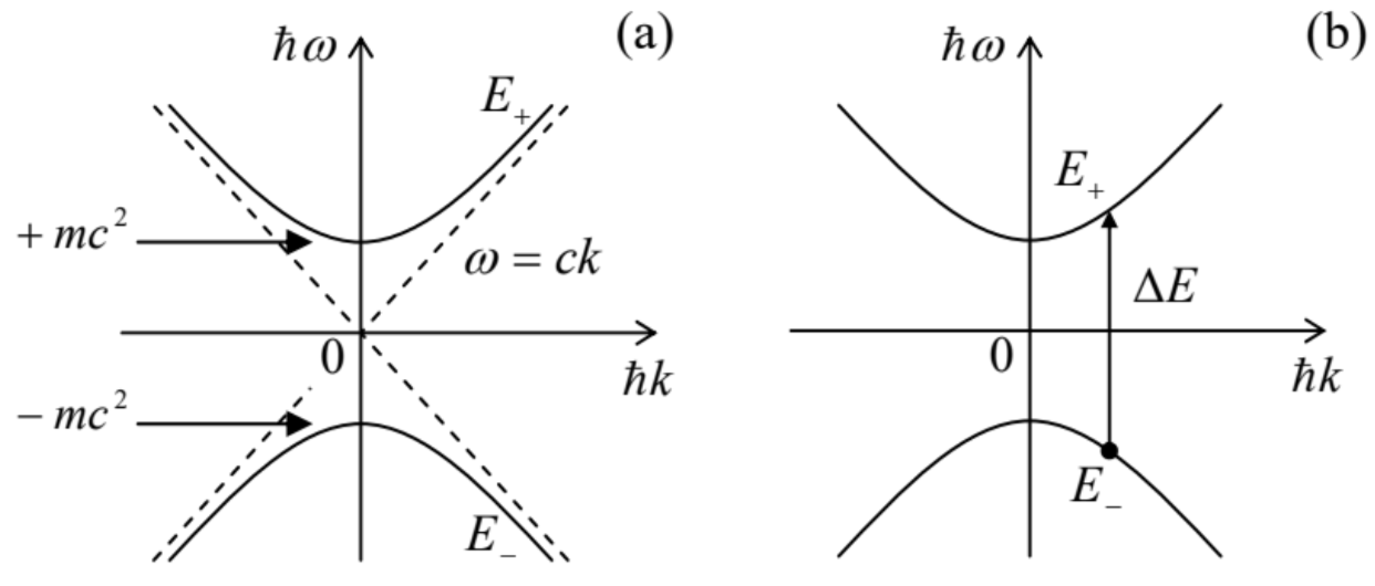 Fig. 9.6. (a) The free-particle dispersion relation resulting from the Klein-Gordon and Dirac equations, and (b) the scheme of creation of a particle-antiparticle pair from the vacuum.
Free particles of a finite spatial extension may be described, in this approach, just as in the nonrelativistic Schrödinger equation, by wave packets, i.e. linear superpositions of the de Broglie waves (85) with close wave vectors k, and the corresponding values of ω given by Eq. (87), with the positive sign for the "usual" particles, and negative sign for antiparticles - see Fig. 6a above. Note that to form, from a particle’s wave packet, a similar wave packet for the antiparticle, with the same phase and group velocities (2.33a) in each direction, we need to change the sign not only before ω, but also before k, i.e. to replace all component wavefunctions (85), and hence the full wavefunction, with their complex conjugates.
Of more formal properties of Eq. (84), it is easy to prove that its solutions satisfy the same continuity equation (1.52), with the probability current density j still given by Eq. (1.47), but a different expression for the probability density w - which becomes very similar to that for j : w=iℏ2mc2(Ψ∗∂Ψ∂t− c.c. ),j=iℏ2m(Ψ∇Ψ∗− c.c. ) - very much in the spirit of the relativity theory, treating space and time on equal footing. (In the nonrelativistic limit p/mc→0, Eq. (84) allows the reduction of this expression for w to the non-relativistic Eq. (1.22): w→ΨΨ∗.)
The Klein-Gordon equation may be readily generalized to describe a particle moving in external fields; for example, the electromagnetic field effects on a particle with charge q may be described by the same replacement as in the non-relativistic limit (see Sec. 3.1): ˆp→ˆP−qA(r,t),ˆH→ˆH−qϕ(r,t), where ˆP=−iℏ∇ is the canonical momentum operator (3.25), and the vector- and scalar potentials, A and ϕ, should be treated appropriately - either as c-number functions if the electromagnetic field quantization is not important for the particular problem, or as operators (see Secs. 1-4 above) if it is.
However, the practical value of the resulting relativistic Schrödinger equation is rather limited, for two main reasons. First of all, it does not give the correct description of particles with spin. For example, for the hydrogen-like atom/ion problem, i.e. the motion of an electron with the electric charge −e, in the Coulomb central field of an immobile nucleus with charge +Ze, the equation may be readily solved exactly 50 and yields the following spectrum of (doubly-degenerate) energy levels: E=mc2(1+Z2α2λ2)−1/2, with λ≡n+[(l+1/2)2−Z2α2]1/2−(l+1/2), where n=1,2,… and l=0,1,…,n−1 are the same quantum numbers as in the non-relativistic theory (see Sec. 3.6), and α≈1/137 is the fine structure constant (6.62). The three leading terms of the Taylor expansion of this result in the small parameter Zα are as follows: E≈mc2[1−Z2α22n2−Z4α42n4(nl+1/2−34)]. The first of these terms is just the rest energy of the particle. The second term, En=−mc2Z2α22n2≡−mZ2e4(4πε0)2ℏ212n2≡−E02n2, with E0=Z2EH, reproduces the non-relativistic Bohr’s formula (3.201). Finally, the third term, −mc2Z4α42n4(nl+1/2−34)≡−2E2nmc2(nl+1/2−34), is just the perturbative kinetic-relativistic contribution (6.51) to the fine structure of the Bohr levels (93). However, as we already know from Sec. 6.3, for a spin-1/2 particle such as the electron, the spin-orbit interaction (6.55) gives an additional contribution to the fine structure, of the same order, so that the net result, confirmed by experiment, is given by Eq. (6.60), i.e. is different from Eq. (94). This is very natural, because the relativistic Schrödinger equation does not have the very notion of spin.
Second, even for massive spinless particles (such as the Z0 bosons), for which this equation is believed to be valid, the most important problems are related to particle interactions at high energies of the order of ΔE∼2mc2 and beyond - see Eq. (88). Due to the possibility of creation and annihilation of particle-antiparticle pairs at such energies, the number of particles participating in such interactions is typically considerable (and variable), and the adequate description of the system is given not by the relativistic Schrödinger equation (which is formulated in single-particle terms), but by the quantum field theory - to which I will devote only a few sentences in the very end of this chapter.
47 This approach was suggested in 1926-1927, i.e. virtually simultaneously, by (at least) V. Fock, E. Schrödinger, O. Klein and W. Gordon, J. Kudar, T. de Donder and F.-H. van der Dungen, and L. de Broglie.
48 Note that in the left, non-relativistic column of this table, the energy is referred to the rest energy mc2, while in its right, relativistic column, it is referred to zero - see Eq. (1).
49 Due to the same P. A. M. Dirac!
50 This task is left for the reader’s exercise.