4.1: Bound Problems


- Last updated
- Mar 4, 2022
- Save as PDF

( \newcommand{\kernel}{\mathrm{null}\,}\)
In the previous chapter we studied stationary problems in which the system is best described as a (time-independent) wave, “scattering” and “tunneling” (that is, showing variation on its intensity) because of obstacles given by changes in the potential energy.
Although the potential determined the space-dependent wavefunction, there was no limitation imposed on the possible wavenumbers and energies involved. An infinite number of continuous energies were possible solutions to the time- independent Schrödinger equation.
In this chapter, we want instead to describe systems which are best described as particles confined inside a potential. This type of system well describe atoms or nuclei whose constituents are bound by their mutual interactions. We shall see that because of the particle confinement, the solutions to the energy eigenvalue equation (i.e. the time- independent Schrödinger equation) are now only a discrete set of possible values (a discrete set os energy levels). The energy is therefore quantized. Correspondingly, only a discrete set of eigenfunctions will be solutions, thus the system, if it’s in a stationary state, can only be found in one of these allowed eigenstates.
We will start to describe simple examples. However, after learning the relevant concepts (and mathematical tricks) we will see how these same concepts are used to predict and describe the energy of atoms and nuclei. This theory can predict for example the discrete emission spectrum of atoms and the nuclear binding energy.
Energy in Square infinite well (particle in a box)
The simplest system to be analyzed is a particle in a box: classically, in 3D, the particle is stuck inside the box and can never leave. Another classical analogy would be a ball at the bottom of a well so deep that no matter how much kinetic energy the ball possess, it will never be able to exit the well.
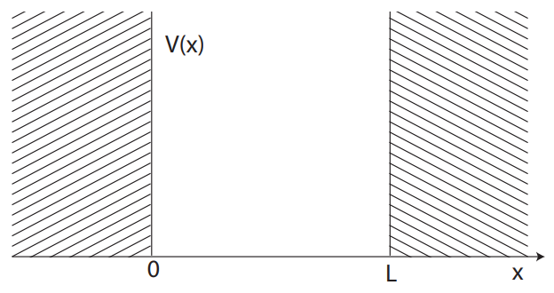
We consider again a particle in a 1D space. However now the particle is no longer free to travel but is confined to be between the positions 0 and L. In order to confine the particle there must be an infinite force at these boundaries that repels the particle and forces it to stay only in the allowed space. Correspondingly there must be an infinite potential in the forbidden region.
Thus the potential function is as depicted in Figure 4.1.2: V(x) = ∞ for x < 0 and x > L; and V(x) = 0 for 0 ≤ x ≤ L. This last condition means that the particle behaves as a free particle inside the well (or box) created by the potential.
We can then write the energy eigenvalue problem inside the well:
H[wn]=−ℏ22m∂2wn(x)∂x2=Enwn(x)
Outside the well we cannot write a proper equation because of the infinities. We can still set the values of wn(x) at the boundaries 0, L. Physically, we expect wn(x)=0 in the forbidden region. In fact, we know that ψ(x)=0 in the forbidden region (since the particle has zero probability of being there)6. Then if we write any ψ(x) in terms of the energy eigenfunctions, ψ(x)=∑ncnwn(x) this has to be zero ∀cn in the forbidden region, thus the wn have to be zero.
At the boundaries we can thus write the boundary conditions7:
wn(0)=wn(L)=0
We can solve the eigenvalue problem inside the well as done for the free particle, obtaining the eigenfunctions
w′n(x)=A′eiknx+B′e−iknx,
with eigenvalues En=ℏ2k2n2m.
It is easier to solve the boundary conditions by considering instead:
wn(x)=Asin(knx)+Bcos(knx)
We have:
wn(0)=A×0+B×1=B=0
Thus from wn(0)=0 we have that B = 0. The second condition states that
wn(L)=Asin(knL)=0
The second condition thus does not set the value of A (that can be done by the normalization condition). In order to satisfy the condition, instead, we have to set
knL=nπ→kn=nπL
for integer n. This condition then in turns sets the allowed values for the energies:
En=ℏ2k2n2m=ℏ2π22mL2n2≡E1n2
where we set E1=ℏ2π22mL2 and n is called a quantum number (associated with the energy eigenvalue). From this, we see that only some values of the energies are allowed. There are still an infinite number of energies, but now they are not a continuous set. We say that the energies are quantized. The quantization of energies (first the photon energies in black-body radiation and photo-electric effect, then the electron energies in the atom) is what gave quantum mechanics its name. However, as we saw from the scattering problems in the previous chapter, the quantization of energies is not a general property of quantum mechanical systems. Although this is common (and the rule any time that the particle is bound, or confined in a region by a potential) the quantization is always a consequence of a particular characteristic of the potential. There exist potentials (as for the free particle, or in general for unbound particles) where the energies are not quantized and do form a continuum (as in the classical case).
6 Note that this is true because the potential is infinite. The energy eigenvalue function (for the Hamiltonian operator) is always valid. The only way for the equation to be valid outside the well it is if wn(x)=0.
7 Note that in this case we cannot require that the first derivative be continuous, since the potential becomes infir boundary. In the cases we examined to describe scattering, the potential had only discontinuity of the first kind.
Finally we calculate the normalization of the energy eigenfunctions:
∫∞−∞dx|wn|2=1→∫L0A2sin(knx)2dx=L2A2=1→A=√2L
Notice that because the system is bound inside a well defined region of space, the normalization condition has now a very clear physical meaning (and thus we must always apply it): if the system is represented by one of the eigenfunctions (and it is thus stationary) we know that it must be found somewhere between 0 and L. Thus the probability of finding the system somewhere in that region must be one. This corresponds to the condition ∫L0p(x)dx=1 or ∫L0|ψ(x)|2dx=1.
Finally, we have
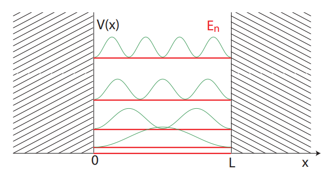
wn(x)=√2Lsinknx,kn=nπL,En=ℏ2π22mL2n2
Now assume that a particle is in an energy eigenstate, that is ψ(x)=wn(x) for some n: ψ(x)=√2Lsin(nπxL). We plot in Figure 4.1.3 some possible wavefunctions.
Consider for example n = 1
Exercise 4.1.1
What does an energy measurement yield? What is the probability of this measurement?
- Answer
-
(E=ℏ2π22m with probability 1)
Exercise 4.1.2
what does a postion measurement yield? What is the probability of finding the particle at 0 ≤ x ≤ L? and at x = 0, L?
Exercise 4.1.3
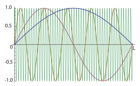
What is the difference in energy between n and n + 1 when n → ∞? And what about the position probability |wn|2 at large n? What does that say about a possible classical limit?
- Answer
-
In the limit of large quantum numbers or small deBroglie wavelength λ∝1/k on average the quantum mechanical description recovers the classical one (Bohr correspondence principle).
Finite Square Well
We now consider a potential which is very similar to the one studied for scattering (compare Figure 3.2.2 to Figure 4.1.4), but that represents a completely different situation. The physical picture modeled by this potential is that of a bound particle. Specifically if we consider the case where the total energy of the particle E2 < 0 is negative, then classically we would expect the particle to be trapped inside the potential well. This is similar to what we already saw when studying the infinite well. Here however the height of the well is finite, so that we will see that the quantum mechanical solution allows for a finite penetration of the wavefunction in the classically forbidden region.
Exercise 4.1.4
What is the expect behavior of a classical particle? (consider for example a snowboarder in a half-pipe. If she does not have enough speed she’s not going to be able to jump over the slope, and will be confined inside)
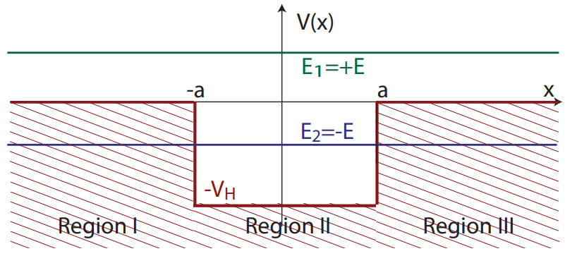
For a quantum mechanical particle we want instead to solve the Schrödinger equation. We consider two cases. In the first case, the kinetic energy is always positive:
Hψ(x)=−2d22mdx2ψ(x)+V(x)ψ(x)=Eψ(x)→{−ℏ22md2ψ(x)dx2=Eψ(x) in Region I −ℏ22md2ψ(x)dx2=(E+VH)ψ(x) in Region II −ℏ22md2ψ(x)dx2=Eψ(x) in Region III
so we expect to find a solution in terms of traveling waves. This is not so interesting, we only note that this describes the case of an unbound particle. The solutions will be similar to scattering solutions (see mathematica demonstration). In the second case, the kinetic energy is greater than zero for |x|≤a and negative otherwise (since the total energy is negative). Notice that I set E to be a positive quantity, and the system’s energy is −E. We also assume that E < VH. The equations are thus rewritten as:
Hψ(x)=−2d22mdx2ψ(x)+V(x)ψ(x)=Eψ(x)→{−ℏ22md2ψ(x)dx2=−Eψ(x) in Region I −ℏ22md2ψ2ψ(x)dx2=(VH−E)ψ(x) in Region II −ℏ22md2ψ(x)dx2=−Eψ(x) in Region III
Then we expect waves inside the well and an imaginary momentum (yielding exponentially decaying probability of finding the particle) in the outside regions. More precisely, in the 3 regions we find:
Region I Region II Region III k′=iκ,k=√2m(VH+E2)ℏ2k′=iκκ=√−2mE2ℏ2=√2mEℏ2=√2m(VH−E)ℏ2κ=√2mEℏ2
And the wavefunction is
Region I Region II Region III C′e−κ|x|A′eikx+B′e−ikxD′e−κx
(Notice that in the first region I can write either C′e−κ|x| or C′eκx. The first notation makes it clear that we have an exponential decay). We now want to match the boundary conditions in order to find the coefficients. Also, we remember from the infinite well that the boundary conditions gave us not the coefficient A, B but a condition on the allowed values of the energy. We expect something similar here, since the infinite case is just a limit of the present case.
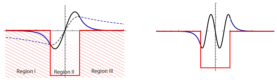
First we note that the potential is an even function of x. The differential operator is also an even function of x. Then the solution has to either be odd or even for the equation to hold. This means that A and B have to be chosen so that ψ(x)=A′eikx+B′e−ikx is either even or odd. This is arranged by setting ψ(x)=Acos(kx) [even solution] or ψ(x)=Asin(kx) [odd solution]. Here I choose the odd solution, ψ(−x)=−ψ(x). That also sets C′=−D′ and we rewrite this constant as −C′=D′=C.
We then have:
Region I Region II Region III ψ(x)=−Ceκxψ(x)=Asin(kx)ψ(x)=Ce−κxψ′(x)=−κCeκxψ′(x)=kAcos(kx)ψ′(x)=−κCe−κx
Since we know that ψ(−x)=−ψ(x) (odd solution) we can consider the boundary matching condition only at x = a.
The two equations are:
{Asin(ka)=Ce−κaAkcos(ka)=−κCe−κa
Substituting the first equation into the second we find: Akcos(ka)=−κAsin(ka). Then we obtain an equation not for the coefficient A (as it was the case for the infinite well) but a constraint on the eigenvalues k and κ:
κ=−kcot(ka)
This is a condition on the eigenvalues that allows only a subset of solutions. This equation cannot be solved analytically, we thus search for a solution graphically (it could be done of course numerically!).
To do so, we first make a change of variable, multiplying both sides by a and setting ka=z,κa=z1. Notice that z21=2mEℏ2a2 and z2=2m(VH−E)ℏ2a2. Setting z20=2mVHa2ℏ2, we have z21=z20−z2 or κa=√z20−z2. Then we can
rewrite the equation κa=−kacot(ka)→z1=−zcot(z) as √z20−z2=−zcot(z), or:
√z20−z2=−zcot(z)
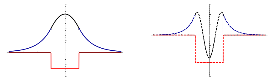
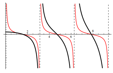
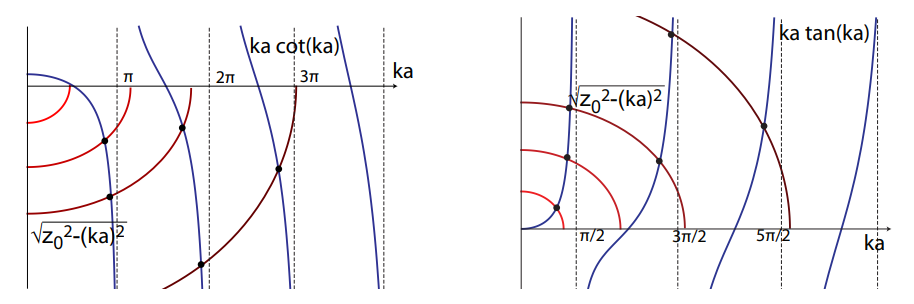
This is a transcendental equation for z (and hence E) as a function of z0, which gives the depth of the well (via VH). To find solutions we plot both sides of the equation and look for crossings. That is, we plot y1(z)=−√z20−z2, which represent a quarter circle (as z is positive) of radius z0=√2mVHa2ℏ2 and y2(z)=zcot(z).
The coefficient A (and thus C and D) can be found (once the eigenfunctions have been found numerically or graphically) by imposing that the eigenfunction is normalized.
Notice that the first red curve never crosses the blue curves. That means that there are no solutions. If z0<π/2 there are no solutions (That is, if the well is too shallow there are no bound solutions, the particle can escape). Only if VH>ℏ2ma2π28 there’s a bound solution.
There’s a finite number of solutions, given a value of z0>π/2. For example, for π/2≤z0≤3π/2 there’s only one solution, 2 for 3π/2≤z0≤5π/2, etc.
Remember however that we only considered the odd solutions. A bound solution is always possible if we consider the even solutions., since the equation to be solved is
κa=katan(ka)=√z20−z2.
Importantly, we found that for the odd solution there is a minimum size of the potential well (width and depth) that supports bound states. How can we estimate this size? A bound state requires a negative total energy, or a kinetic energy smaller than the potential: Ekin=ℏ2k22m<VH. This poses a constraint on the wavenumber k and thus the wavelength, λ=2πk.
λ≥2πℏ√2mVH
However, in order to satisfy the boundary conditions (that connect the oscillating wavefunction to the exponentially decay one) we need to fit at least half of a wavelength inside the 2a width of the potential, 12λ≤2a. Then we obtain