
9.3: Confined Matter Waves


- Last updated
- Nov 6, 2024
- Save as PDF

( \newcommand{\kernel}{\mathrm{null}\,}\)
Confinement of a wave to a limited spatial region results in rather peculiar behavior — the wave can only fit comfortably into the confined region if the wave frequency, and hence the associated particle energy, takes on a limited set of possible values. This is the origin of the famous quantization of energy, from which the “quantum” in quantum mechanics comes. We will explore two types of confinement, position confinement due to a potential energy well, and rotational confinement due to the fact that rotation of an object through 2π radians returns the object to its original orientation.
Particle in a Box
We now imagine how a particle confined to a region 0≤x≤a on the x axis must behave. As with the displacement of a guitar string, the wave function must be zero at x=0 and a, i. e., at the ends of the guitar string. A single complex exponential plane wave cannot satisfy this condition, since |exp[i(kx−ωt)]|2=1 everywhere. However, a superposition (with a minus sign) of leftward and rightward traveling waves creates a standing wave, in which the the wave function separates into a function of space alone times a function of time alone.
ψ=exp[i(kx−ωt)]−exp[i(−kx−ωt)]=2iexp(−iωt)sin(kx)
Notice that the time dependence is still a complex exponential, which means that |Ψ|2 is independent of time. This insures that the probability of finding the particle somewhere in the box remains constant with time. It also means that the wave packet corresponds to a definite energy E=ℏω.
Because we took a difference rather than a sum of plane waves, the condition ψ=0 is already satisfied at x=0. To satisfy it at x=a, we must have ka=nπ, where n=1,2,3,…. Thus, the absolute value of the wave number must take on the discrete values
kn=nπa,n=1,2,3,…
(The wavenumbers of the two plane waves equal plus or minus this absolute value respectively.) This implies that the absolute value of the particle momentum is Πn=ℏkn=nrℏa, which in turn means that the energy of the particle must be
En=(Π2nc2+m2c4)1/2=(n2π2ℏ2c2/a2+m2c4)1/2
where m is the particle mass. In the non-relativistic limit this becomes
En=Π2n2m=n2π2ℏ22ma2 (non-relativistic)
where we have dropped the rest energy mc2 since it is a constant offset. In the ultra-relativistic case where we can ignore the particle mass, we find
En=|Πn|c=nπℏca (zero mass)
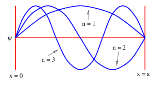
The shapes of the wave functions for the first three values of n for the particle in the box are illustrated in Figure 9.3.2:.
In both limits the energy takes on only a certain set of possible values. This is called energy quantization and the integer n is called the energy quantum number. In the non-relativistic limit the energy is proportional to n2, while in the ultra-relativistic case the energy is proportional to n.
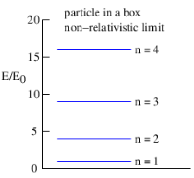
We can graphically represent the allowed energy levels for the particle in a box by an energy level diagram. Such a diagram is shown in Figure 9.3.3: for the non-relativistic case.
One aspect of this problem deserves a closer look. Equation (???) shows that the wave function for this problem is a superposition of two plane waves corresponding to momenta Π1=+ℏk and Π2=−ℏk and is therefore a kind of wave packet. Thus, the wave function is not invariant under displacement and does not correspond to a definite value of the momentum — the momentum’s absolute value is definite, but its sign is not. Following Feynman’s prescription, equation (???) tells us that the amplitude for the particle in the box to have momentum +ℏk is exp[i(kx−ωt)], while the amplitude for it to have momentum −ℏk is −exp[i(−kx−ωt)]. The absolute square of the sum of these amplitudes gives us the relative probability of finding the particle at position x:
P(x)=|2iexp(−iωt)sin(kx)|2=4sin2(kx)
Which of the two possible values of the momentum the particle takes on is unknowable, just as it is impossible in principle to know which slit a particle passes through in two slit interference. If an experiment is done to measure the momentum, then the wave function is irreversibly changed, just as the interference pattern in the two slit problem is destroyed if the slit through which the particle passes is unambiguously determined.
Barrier Penetration
Unlike the situation in classical mechanics, quantum mechanics allows the kinetic energy K to be negative. This makes the momentum Π( equal to (2mK)1/2 in the nonrelativistic case) imaginary, which in turn gives rise to an imaginary wavenumber.
Let us investigate the nature of a wave with an imaginary wavenumber. Let us assume that k=iκ in a complex exponential plane wave, where κ is real:
ψ=exp[i(kx−ωt)]=exp(−κx−iωt)=exp(−κx)exp(−iωt)
The wave function doesn’t oscillate in space when K=E−U<0, but grows or decays exponentially with x, depending on the sign of κ.
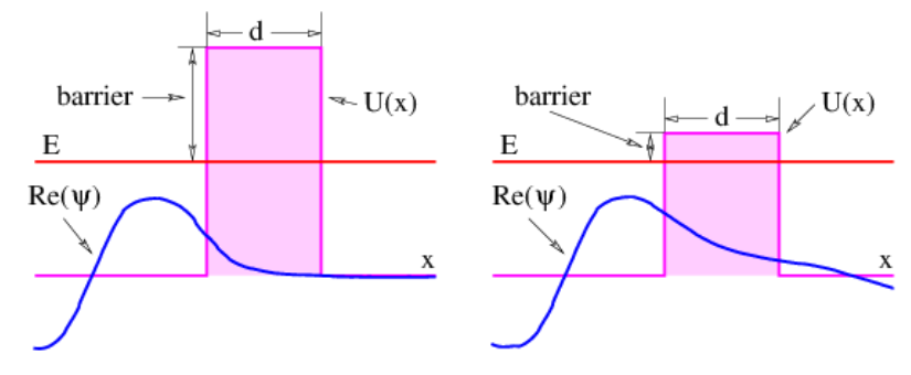
For a particle moving to the right, with positive k in the allowed region, κ turns out to be positive, and the solution decays to the right. Thus, a particle impingent on a potential energy barrier from the left (i. e., while moving to the right) will have its wave amplitude decay in the classically forbidden region, as illustrated in Figure 9.3.4:. If this decay is very rapid, then the result is almost indistinguishable from the classical result — the particle cannot penetrate into the forbidden region to any great extent. However, if the decay is slow, then there is a reasonable chance of finding the particle in the forbidden region. If the forbidden region is finite in extent, then the wave amplitude will be small, but non-zero at its right boundary, implying that the particle has a finite chance of completely passing through the classical forbidden region. This process is called barrier penetration.
The probability for a particle to penetrate a barrier is the absolute square of the amplitude after the barrier divided by the square of the amplitude before the barrier. Thus, in the case of the wave function illustrated in equation (???), the probability of penetration is
P=|ψ(d)|2/|ψ(0)|2=exp(−2κd)
where d is the thickness of the barrier.
The rate of exponential decay with x in the forbidden region is related to how negative K is in this region. Since
−K=U−E=−Π22m=−ℏ2k22m=ℏ2κ22m
we find that
κ=(2mBℏ2)1/2
where the potential energy barrier is B≡−K=U−E. The smaller B is, the smaller is κ, resulting in less rapid decay of the wave function with x. This corresponds to stronger barrier penetration. (Note that the way B is defined, it is positive in forbidden regions.)
If the energy barrier is very high, then the exponential decay of the wave function is very rapid. In this case the wave function goes nearly to zero at the boundary between the allowed and forbidden regions. This is why we specify the wave function to be zero at the walls for the particle in a box. These walls act in effect as infinitely high potential barriers.
Barrier penetration is important in a number of natural phenomena. Certain types of radioactive decay and the fissioning of heavy nuclei are governed by this process.
Orbital Angular Momentum
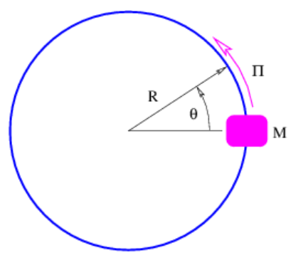
Another type of bound state motion occurs when a particle is constrained to move in a circle. (Imagine a bead sliding on a circular loop of wire, as illustrated in Figure 9.3.5:.) We can define x in this case as the path length around the wire and relate it to the angle θ:x=Rθ. For a plane wave we have
ψ=exp[i(kx−ωt)]=exp[i(kRθ−ωt)]
This plane wave differs from the normal plane wave for motion along a Cartesian axis in that we must have ψ(θ)=ψ(θ+2π). This can only happen if the circumference of the loop, 2πR, is an integral number of wavelengths, i. e., if 2πR/λ=m where m is an integer. However, since 2Π/λ=k, this condition becomes kR=m.
Since Π=ℏk, the above condition can be written ΠmR=mℏ. The quantity
Lm≡ΠmR
is called the angular momentum, leading to our final result,
Lm=mℏ,m=0,±1,±2,…
We see that the angular momentum can only take on values which are integer multiples of ℏ. This represents the quantization of angular momentum, and m in this case is called the angular momentum quantum number. Note that this quantum number differs from the energy quantum number for the particle in the box in that zero and negative values are allowed.
The energy of our bead on a loop of wire can be expressed in terms of the angular momentum:
Em=Π2m2M=L2m2MR2
This means that angular momentum and energy are compatible variables in this case, which further means that angular momentum is a conserved variable. Just as definite values of linear momentum are related to invariance under translations, definite values of angular momentum are related to invariance under rotations. Thus, we have
invariance under rotation ⟺ definite angular momentum
for angular momentum.
We need to briefly address the issue of angular momentum in three dimensions. Angular momentum is actually a vector oriented perpendicular to the wire loop in the example we are discussing. The direction of the vector is defined using a variation on the right-hand rule: Curl your fingers in the direction of motion of the bead around the loop (using your right hand!). The orientation of the angular momentum vector is defined by the direction in which your thumb points. This tells you, for instance, that the angular momentum in Figure 9.3.5: points out of the page.
In quantum mechanics it is only possible to measure simultaneously the square of the length of the angular momentum vector and one component of this vector. Two different components of angular momentum cannot be simultaneously measured because of the uncertainty principle. However, the length of the angular momentum vector may be measured simultaneously with one component. Thus, in quantum mechanics, the angular momentum is completely specified if the length and one component of the angular momentum vector are known.
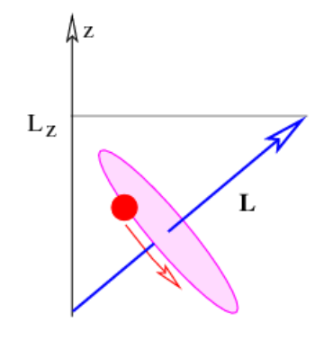
Figure 9.6 illustrates the angular momentum vector associated with a bead moving on a wire loop which is tilted from the horizontal. One component (taken to be the z component) is shown as well. For reasons we cannot explore here, the square of the length of the angular momentum vector L2 is quantized with the following values:
L2l=ℏ2l(l+1),l=0,1,2,…
One component (say, the z component) of angular momentum is quantized just like angular momentum in the two-dimensional case, except that l acts as an upper bound on the possible values of |m|. In other words, if the square of the length of the angular momentum vector is ℏ2∣(∣+1), then the z component can take on the values
Lzm=ℏm,m=−l,−l+1,…,l−1,l
The quantity l is called the angular momentum quantum number, while m is called the orientation or magnetic quantum number, the latter for historical reasons.
Angular Momentum
The type of angular momentum discussed above is associated with the movement of particles in orbits. However, it turns out that even stationary particles can possess angular momentum. This is called spin angular momentum. The spin quantum number s plays a role analogous to l for spin angular momentum, i. e., the square of the spin angular momentum vector of a particle is
L2s=ℏ2s(s+1)
The spin orientation quantum number ms is similarly related to s:
Lzs=ℏms,ms=−s,−s+1,…,s−1,s
The spin angular momentum for an elementary particle is absolutely conserved, i. e., it can never change. Thus, the value of s is an intrinsic property of a particle. The major difference between spin and orbital angular momentum is that the spin quantum number can take on more values, i. e., s=0,1/2,1,3/2,2,5/2,…
Particles with integer spin values s=0,1,2,… are called bosons after the Indian physicist Satyendra Nath Bose. Particles with half-integer spin values s=1/2,3/2,5/2,… are called fermions after the Italian physicist Enrico Fermi. As we shall see later in the course, bosons and fermions play very different roles in the universe.