7.2: Beta Decay
- Page ID
- 25732
\( \newcommand{\vecs}[1]{\overset { \scriptstyle \rightharpoonup} {\mathbf{#1}} } \)
\( \newcommand{\vecd}[1]{\overset{-\!-\!\rightharpoonup}{\vphantom{a}\smash {#1}}} \)
\( \newcommand{\dsum}{\displaystyle\sum\limits} \)
\( \newcommand{\dint}{\displaystyle\int\limits} \)
\( \newcommand{\dlim}{\displaystyle\lim\limits} \)
\( \newcommand{\id}{\mathrm{id}}\) \( \newcommand{\Span}{\mathrm{span}}\)
( \newcommand{\kernel}{\mathrm{null}\,}\) \( \newcommand{\range}{\mathrm{range}\,}\)
\( \newcommand{\RealPart}{\mathrm{Re}}\) \( \newcommand{\ImaginaryPart}{\mathrm{Im}}\)
\( \newcommand{\Argument}{\mathrm{Arg}}\) \( \newcommand{\norm}[1]{\| #1 \|}\)
\( \newcommand{\inner}[2]{\langle #1, #2 \rangle}\)
\( \newcommand{\Span}{\mathrm{span}}\)
\( \newcommand{\id}{\mathrm{id}}\)
\( \newcommand{\Span}{\mathrm{span}}\)
\( \newcommand{\kernel}{\mathrm{null}\,}\)
\( \newcommand{\range}{\mathrm{range}\,}\)
\( \newcommand{\RealPart}{\mathrm{Re}}\)
\( \newcommand{\ImaginaryPart}{\mathrm{Im}}\)
\( \newcommand{\Argument}{\mathrm{Arg}}\)
\( \newcommand{\norm}[1]{\| #1 \|}\)
\( \newcommand{\inner}[2]{\langle #1, #2 \rangle}\)
\( \newcommand{\Span}{\mathrm{span}}\) \( \newcommand{\AA}{\unicode[.8,0]{x212B}}\)
\( \newcommand{\vectorA}[1]{\vec{#1}} % arrow\)
\( \newcommand{\vectorAt}[1]{\vec{\text{#1}}} % arrow\)
\( \newcommand{\vectorB}[1]{\overset { \scriptstyle \rightharpoonup} {\mathbf{#1}} } \)
\( \newcommand{\vectorC}[1]{\textbf{#1}} \)
\( \newcommand{\vectorD}[1]{\overrightarrow{#1}} \)
\( \newcommand{\vectorDt}[1]{\overrightarrow{\text{#1}}} \)
\( \newcommand{\vectE}[1]{\overset{-\!-\!\rightharpoonup}{\vphantom{a}\smash{\mathbf {#1}}}} \)
\( \newcommand{\vecs}[1]{\overset { \scriptstyle \rightharpoonup} {\mathbf{#1}} } \)
\(\newcommand{\longvect}{\overrightarrow}\)
\( \newcommand{\vecd}[1]{\overset{-\!-\!\rightharpoonup}{\vphantom{a}\smash {#1}}} \)
\(\newcommand{\avec}{\mathbf a}\) \(\newcommand{\bvec}{\mathbf b}\) \(\newcommand{\cvec}{\mathbf c}\) \(\newcommand{\dvec}{\mathbf d}\) \(\newcommand{\dtil}{\widetilde{\mathbf d}}\) \(\newcommand{\evec}{\mathbf e}\) \(\newcommand{\fvec}{\mathbf f}\) \(\newcommand{\nvec}{\mathbf n}\) \(\newcommand{\pvec}{\mathbf p}\) \(\newcommand{\qvec}{\mathbf q}\) \(\newcommand{\svec}{\mathbf s}\) \(\newcommand{\tvec}{\mathbf t}\) \(\newcommand{\uvec}{\mathbf u}\) \(\newcommand{\vvec}{\mathbf v}\) \(\newcommand{\wvec}{\mathbf w}\) \(\newcommand{\xvec}{\mathbf x}\) \(\newcommand{\yvec}{\mathbf y}\) \(\newcommand{\zvec}{\mathbf z}\) \(\newcommand{\rvec}{\mathbf r}\) \(\newcommand{\mvec}{\mathbf m}\) \(\newcommand{\zerovec}{\mathbf 0}\) \(\newcommand{\onevec}{\mathbf 1}\) \(\newcommand{\real}{\mathbb R}\) \(\newcommand{\twovec}[2]{\left[\begin{array}{r}#1 \\ #2 \end{array}\right]}\) \(\newcommand{\ctwovec}[2]{\left[\begin{array}{c}#1 \\ #2 \end{array}\right]}\) \(\newcommand{\threevec}[3]{\left[\begin{array}{r}#1 \\ #2 \\ #3 \end{array}\right]}\) \(\newcommand{\cthreevec}[3]{\left[\begin{array}{c}#1 \\ #2 \\ #3 \end{array}\right]}\) \(\newcommand{\fourvec}[4]{\left[\begin{array}{r}#1 \\ #2 \\ #3 \\ #4 \end{array}\right]}\) \(\newcommand{\cfourvec}[4]{\left[\begin{array}{c}#1 \\ #2 \\ #3 \\ #4 \end{array}\right]}\) \(\newcommand{\fivevec}[5]{\left[\begin{array}{r}#1 \\ #2 \\ #3 \\ #4 \\ #5 \\ \end{array}\right]}\) \(\newcommand{\cfivevec}[5]{\left[\begin{array}{c}#1 \\ #2 \\ #3 \\ #4 \\ #5 \\ \end{array}\right]}\) \(\newcommand{\mattwo}[4]{\left[\begin{array}{rr}#1 \amp #2 \\ #3 \amp #4 \\ \end{array}\right]}\) \(\newcommand{\laspan}[1]{\text{Span}\{#1\}}\) \(\newcommand{\bcal}{\cal B}\) \(\newcommand{\ccal}{\cal C}\) \(\newcommand{\scal}{\cal S}\) \(\newcommand{\wcal}{\cal W}\) \(\newcommand{\ecal}{\cal E}\) \(\newcommand{\coords}[2]{\left\{#1\right\}_{#2}}\) \(\newcommand{\gray}[1]{\color{gray}{#1}}\) \(\newcommand{\lgray}[1]{\color{lightgray}{#1}}\) \(\newcommand{\rank}{\operatorname{rank}}\) \(\newcommand{\row}{\text{Row}}\) \(\newcommand{\col}{\text{Col}}\) \(\renewcommand{\row}{\text{Row}}\) \(\newcommand{\nul}{\text{Nul}}\) \(\newcommand{\var}{\text{Var}}\) \(\newcommand{\corr}{\text{corr}}\) \(\newcommand{\len}[1]{\left|#1\right|}\) \(\newcommand{\bbar}{\overline{\bvec}}\) \(\newcommand{\bhat}{\widehat{\bvec}}\) \(\newcommand{\bperp}{\bvec^\perp}\) \(\newcommand{\xhat}{\widehat{\xvec}}\) \(\newcommand{\vhat}{\widehat{\vvec}}\) \(\newcommand{\uhat}{\widehat{\uvec}}\) \(\newcommand{\what}{\widehat{\wvec}}\) \(\newcommand{\Sighat}{\widehat{\Sigma}}\) \(\newcommand{\lt}{<}\) \(\newcommand{\gt}{>}\) \(\newcommand{\amp}{&}\) \(\definecolor{fillinmathshade}{gray}{0.9}\)The beta decay is a radioactive decay in which a proton in a nucleus is converted into a neutron (or vice-versa). In the process the nucleus emits a beta particle (either an electron or a positron) and quasi-massless particle, the neutrino.
Recall the mass chain and Beta decay plots of Fig. 7. When studying the binding energy from the SEMF we saw that at fixed A there was a minimum in the nuclear mass for a particular value of Z. In order to reach that minimum, unstable nuclides undergo beta decay to transform excess protons in neutrons (and vice-versa).
Reactions and Phenomenology
The beta-decay reaction is written as:
\[\ce{_{Z}^{A} X_{N} -> _{Z+1}^{A} X_{N-1}^{\prime} + e^{-} + \bar{\nu}} \nonumber\]
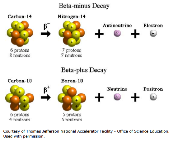
This is the \(\beta^{-}\) decay. (or negative beta decay) The underlying reaction is:
\[\ce{n \rightarrow p + e^{-} + \bar{\nu}} \nonumber\]
which converts a proton into a neutron with the emission of an electron and an anti-neutrino. There are two other types of reactions, the \(\beta^{+}\) reaction,
\[\ce{ ^{A}_{Z} X_{N} -> _{Z-1}^{A} X_{N+1}^{\prime} + e^{+} + \nu } \nonumber\]
with this underlying reaction
\[\ce{p -> n + e^{+} + \nu} \nonumber\]
which sees the emission of a positron (the electron anti-particle) and a neutrino; and the electron capture:
\[{ }_{Z}^{A} X_{N}+e^{-} \rightarrow{ }_{Z-1}^{A} X_{N+1}^{\prime}+\nu \nonumber\]
with this underlying reaction
\[\ce{ p + e^{-} \rightarrow n+\nu} \nonumber\]
a process that competes with, or substitutes, the positron emission.
\[{ }_{29}^{64} \mathrm{Cu} \backslash \begin{array}{ll}
\nearrow & { }^{64} \mathrm{Zn}+e^{-}+\bar{\nu}, \quad Q_{\beta}=0.57 M \mathrm{eV} \\
& { }_{28}^{64} \mathrm{Ni}+e^{+}+\nu, \quad Q_{\beta}=0.66 \mathrm{MeV}
\end{array} \nonumber\]
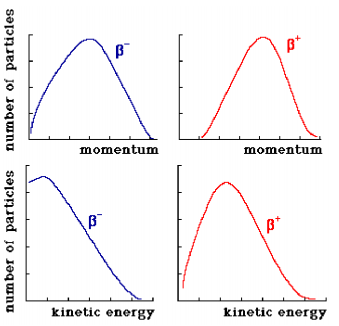
The neutrino and beta particle (\(\beta^{\pm}\)) share the energy.
Since the neutrinos are very difficult to detect (as we will see they are almost massless and interact very weakly with matter), the electrons/positrons are the particles detected in beta-decay and they present a characteristic energy spectrum (see Fig. 45). The difference between the spectrum of the \(\beta^{\pm}\) particles is due to the Coulomb repulsion or attraction from the nucleus. Notice that the neutrinos also carry away angular momentum. They are spin-1/2 particles, with no charge (hence the name) and very small mass. For many years it was actually believed to have zero mass. However it has been confirmed that it does have a mass in 1998.
Conservation Laws
As the neutrino is hard to detect, initially the beta decay seemed to violate energy conservation. Introducing an extra particle in the process allows one to respect conservation of energy. Besides energy, there are other conserved quantities:
- Energy: The Q value of a beta decay is given by the usual formula:
\[Q_{\beta^{-}}=\left[m_{N}\left({ }^{A} X\right)-m_{N}\left({ }_{Z+1}^{A} X^{\prime}\right)-m_{e}\right] c^{2}. \nonumber\]
Using the atomic masses and neglecting the electron’s binding energies as usual we have
\[\begin{align*} Q_{\beta^{-}} &=\left\{\left[m_{A}\left({ }^{A} X\right)-Z m_{e}\right]-\left[m_{A}\left({ }_{Z+1}^{A} X^{\prime}\right)-(Z+1) m_{e}\right]-m_{e}\right\} c^{2} \\[4pt] &=\left[m_{A}\left({ }^{A} X\right)-m_{A}\left({ }_{Z+1}^{A} X^{\prime}\right)\right] c^{2}. \end{align*}\]
The kinetic energy (equal to the \(Q\)) is shared by the neutrino and the electron (we neglect any recoil of the massive nucleus). Then, the emerging electron (remember, the only particle that we can really observe) does not have a fixed energy, as it was for example for the gamma photon. But it will exhibit a spectrum of energy (which is the number of electron at a given energy) as well as a distribution of momenta. We will see how we can reproduce these plots by analyzing the QM theory of beta decay.
- Momentum: The momentum is also shared between the electron and the neutrino. Thus the observed electron momentum ranges from zero to a maximum possible momentum transfer.
- Angular momentum (both the electron and the neutrino have spin 1/2)
- Parity? It turns out that parity is not conserved in this decay. This hints to the fact that the interaction responsible violates parity conservation (so it cannot be the same interactions we already studies, e.m. and strong interactions)
- Charge (thus the creation of a proton is for example always accompanied by the creation of an electron)
- Lepton number: we do not conserve the total number of particles (we create beta and neutrinos). However the number of massive, heavy particles (or baryons, composed of 3 quarks) is conserved. Also the lepton number is conserved. Leptons are fundamental particles (including the electron, muon and tau, as well as the three types of neutrinos associated with these 3). The lepton number is +1 for these particles and -1 for their antiparticles. Then an electron is always accompanied by the creation of an antineutrino, e.g., to conserve the lepton number (initially zero).
Fermi’s Theory of Beta Decay
The properties of beta decay can be understood by studying its quantum-mechanical description via Fermi’s Golden rule, as done for gamma decay.
\[W=\frac{2 \pi}{\hbar}\left|\left\langle\psi_{f}|\hat{V}| \psi_{i}\right\rangle\right|^{2} \rho\left(E_{f}\right) \nonumber\]
In gamma decay process we have seen how the e.m. field is described as an operator that can create (or destroy) photons. Nobody objected to the fact that we can create this massless particles. After all, we are familiar with charged particles that produce (create) an e.m. field. However in QM photons are also particles, and by analogy we can have also creation of other types of particles, such as the electron and the neutrino.
For the beta decay we need another type of interaction that is able to create massive particles (the electron and neutrino). The interaction cannot be given by the e.m. field; moreover, in the light of the possibilities of creating and annihilating particles, we also need to find a new description for the particles themselves that allows these processes. All of this is obtained by quantum field theory and the second quantization. Quantum field theory gives a unification of e.m. and weak force (electro-weak interaction) with one coupling constant e. The interaction responsible for the creation of the electron and neutrino in the beta decay is called the weak interaction and its one of the four fundamental interactions (together with gravitation, electromagnetism and the strong interaction that keeps nucleons and quarks together). One characteristic of this interaction is parity violation.
Matrix element
The weak interaction can be written in terms of the particle field wavefunctions:
\[V_{i n t}=g \Psi_{e}^{\dagger} \Psi_{\bar{\nu}}^{\dagger} \nonumber\]
where \(\Psi_{a}\left(\Psi_{a}^{\dagger}\right)\) annihilates (creates) the particle a, and g is the coupling constant that determines how strong the interaction is. Remember that the analogous operator for the e.m. field was \(\propto a_{k}^{\dagger}\) (creating one photon of momentum k).
Then the matrix element
\[V_{i f}=\left\langle\psi_{f}\left|\mathcal{H}_{i n t}\right| \psi_{i}\right\rangle \nonumber\]
can be written as:
\[V_{i f}=g \int d^{3} \vec{x} \Psi_{p}^{*}(\vec{x})\left[\Psi_{e}^{*}(\vec{x}) \Psi_{\bar{\nu}}^{*}(\vec{x})\right] \Psi_{n}(\vec{x}) \nonumber\]
(Here \(\dagger \rightarrow *\) since we have scalar operators).
To first approximation the electron and neutrino can be taken as plane waves:
\[V_{i f}=g \int d^{3} \vec{x} \Psi_{p}^{*}(\vec{x}) \frac{e^{i \vec{k}_{e} \cdot \vec{x}}}{\sqrt{V}} \frac{e^{i \vec{k}_{\nu} \cdot \vec{x}}}{\sqrt{V}} \Psi_{n}(\vec{x}) \nonumber\]
and since \(k R \ll 1\) we can approximate this with
\[V_{i f}=\frac{g}{V} \int d^{3} \vec{x} \Psi_{p}^{*}(\vec{x}) \Psi_{n}(\vec{x}) \nonumber\]
We then write this matrix element as
\[V_{i f}=\frac{g}{V} M_{n p} \nonumber\]
where \(M_{n p}\) is a very complicated function of the nuclear spin and angular momentum states. In addition, we will use in the Fermi’s Golden Rule the expression
\[\left|M_{n p}\right|^{2} \rightarrow\left|M_{n p}\right|^{2} F\left(Z_{0}, Q_{\beta}\right) \nonumber\]
where the Fermi function \(F\left(Z_{0}, Q_{\beta}\right)\) accounts for the Coulomb interaction between the nucleus and the electron that we had neglected in the previous expression (where we only considered the weak interaction).
Density of states
In studying the gamma decay we calculated the density of states, as required by the Fermi’s Golden Rule. Here we need to do the same, but the problem is complicated by the fact that there are two types of particles (electron and neutrino) as products of the reaction and both can be in a continuum of possible states. Then the number of states in a small energy volume is the product of the electron and neutrino’s states:
\[d^{2} N_{s}=d N_{e} d N_{\nu}. \nonumber\]
The two particles share the \(Q\) energy:
\[Q_{\beta}=T_{e}+T_{\nu}. \nonumber\]
For simplicity we assume that the mass of the neutrino is zero (it’s much smaller than the electron mass and of the kinetic mass of the neutrino itself). Then we can take the relativistic expression
\[T_{\nu}=c p_{\nu}, \nonumber\]
while for the electron
\[E^{2}=p^{2} c^{2}+m^{2} c^{4} \quad \rightarrow \quad E=T_{e}+m_{e} c^{2} \quad \text { with } T_{e}=\sqrt{p_{e}^{2} c^{2}+m_{e}^{2} c^{4}}-m_{e} c^{2} \nonumber\]
and we then write the kinetic energy of the neutrino as a function of the electron's,
\[T_{\nu}=Q_{\beta}-T_{e}. \nonumber\]
The number of states for the electron can be calculated from the quantized momentum, under the assumption that the electron state is a free particle \(\left(\psi \sim e^{i \vec{k} \cdot \vec{r}}\right)\) in a region of volume \(V=L^{3}:\)
\[d N_{e}=\left(\frac{L}{2 \pi}\right)^{3} 4 \pi k_{e}^{2} d k_{e}=\frac{4 \pi V}{(2 \pi \hbar)^{3}} p_{e}^{2} d p_{e} \nonumber\]
and the same for the neutrino,
\[d N_{\nu}=\frac{4 \pi V}{(2 \pi \hbar)^{3}} p_{\nu}^{2} d p_{\nu} \nonumber\]
where we used the relationship between momentum and wavenumber: \(\vec{p}=\hbar \vec{k}.\)
At a given momentum/energy value for the electron, we can write the density of states as
\[\rho\left(p_{e}\right) d p_{e}=d N_{e} \frac{d N_{\nu}}{d T_{\nu}}=16 \pi^{2} \frac{V^{2}}{(2 \pi \hbar)^{6}} p_{e}^{2} d p_{e} p_{\nu}^{2} \frac{d p_{\nu}}{d T_{\nu}}=\frac{V^{2}}{4 \pi^{4} \hbar^{6} c^{3}}\left[Q-T_{e}\right]^{2} p_{e}^{2} d p_{e} \nonumber\]
where we used : \(\frac{d T_{\nu}}{d p_{\nu}}=c\) and \(p_{\nu}=\left(Q_{\beta}-T_{e}\right) / c.\)
The density of states is then
\[\rho\left(p_{e}\right) d p_{e}=\frac{V^{2}}{4 \pi^{4} \hbar^{6} c^{3}}\left[Q-T_{e}\right]^{2} p_{e}^{2} d p_{e}=\frac{V^{2}}{4 \pi^{4} \hbar^{6} c^{3}}\left[Q-\left(\sqrt{p_{e}^{2} c^{2}+m_{e}^{2} c^{4}}-m_{e} c^{2}\right)\right]^{2} p_{e}^{2} d p_{e} \nonumber\]
or rewriting this expression in terms of the electron kinetic energy:
\[\rho\left(T_{e}\right)=\frac{V^{2}}{4 \pi^{4} \hbar^{6} c^{3}}\left[Q-T_{e}\right]^{2} p_{e}^{2} \frac{d p_{e}}{d T_{e}}=\frac{V^{2}}{4 c^{6} \pi^{4} \hbar^{6}}\left[Q-T_{e}\right]^{2} \sqrt{T_{e}^{2}+2 T_{e} m_{e} c^{2}}\left(T_{e}+m_{e} c^{2}\right) \nonumber\]
\(\left(\text { as } p_{e} d p_{e}=\left(T_{e}+m_{e} c^{2}\right) / c^{2} d T_{e}\right)\)
Knowing the density of states, we can calculate how many electrons are emitted in the beta decay with a given energy. This will be proportional to the rate of emission calculated from the Fermi Golden Rule, times the density of states:
\[N(p)=C F(Z, Q)\left|V_{f i}\right|^{2} \frac{p^{2}}{c^{2}}[Q-T]^{2}=C F(Z, Q)\left|V_{f i}\right|^{2} \frac{p^{2}}{c^{2}}\left[Q-\left(\sqrt{p_{e}^{2} c^{2}+m_{e}^{2} c^{4}}-m_{e} c^{2}\right)\right]^{2} \nonumber\]
and
\[N\left(T_{e}\right)=\frac{C}{c^{5}} F(Z, Q)\left|V_{f i}\right|^{2}\left[Q-T_{e}\right]^{2} \sqrt{T_{e}^{2}+2 T_{e} m_{e} c^{2}}\left(T_{e}+m_{e} c^{2}\right) \nonumber\]
These distributions are nothing else than the spectrum of the emitted beta particles (electron or positron). In these expression we collected in the constant C various parameters deriving from the Fermi Golden Rule and density of states calculations, since we want to highlight only the dependence on the energy and momentum. Also, we introduced a new function, F(Z, Q), called the Fermi function, that takes into account the shape of the nuclear wavefunction and in particular it describes the Coulomb attraction or repulsion of the electron or positron from the nucleus. Thus, F(Z, Q) is different, depending on the type of decay. These distributions were plotted in Fig. 45. Notice that these distributions (as well as the decay rate below) are the product of three terms:
- the Statistical factor (arising from the density of states calculation), \(\frac{p^{2}}{c^{2}}[Q-T]^{2}\)
- the Fermi function (accounting for the Coulomb interaction), F(Z, Q)
- and the Transition amplitude from the Fermi Golden Rule, \(\left|V_{f i}\right|^{2}\)
These three terms reflect the three ingredients that determine the spectrum and decay rate of in beta decay processes.
Decay rate
The decay rate is obtained from Fermi’s Golden rule:
\[W=\frac{2 \pi}{\hbar}\left|V_{i f}\right|^{2} \rho(E) \nonumber\]
where ρ(E) is the total density of states. ρ(E) (and thus the decay rate) is obtained by summing over all possible states of the beta particle, as counted by the density of states. Thus, in practice, we need to integrate the density of states over all possible momentum of the outgoing electron/positron. Upon integration over \(p_{e}\) we obtain:
\[\rho(E)=\frac{V^{2}}{4 \pi^{4} \hbar^{6} c^{3}} \int_{0}^{p_{e}^{m a x}} d p_{e}\left[Q-T_{e}\right]^{2} p_{e}^{2} \approx \frac{V^{2}}{4 \pi^{4} \hbar^{6} c^{3}} \frac{\left(Q-m c^{2}\right)^{5}}{30 c^{3}} \nonumber\]
(where we took \(T_{e} \approx p c\) in the relativistic limit for high electron speed).
We can finally write the decay rate as:
\[W=\frac{2 \pi}{\hbar}\left|V_{i f}\right|^{2} \rho(E)=\frac{2 \pi}{\hbar} \frac{g}{V}^{2}\left|M_{n p}\right|^{2} F\left(Z, Q_{\beta}\right) \frac{V^{2}}{4 \pi^{4} \hbar^{6} c^{3}} \frac{\left(Q-m c^{2}\right)^{5}}{30 c^{3}} \nonumber\]
\[=G_{F}^{2}\left|M_{n p}\right|^{2} F\left(Z, Q_{\beta}\right) \frac{\left(Q-m c^{2}\right)^{5}}{60 \pi^{3} \hbar(\hbar c)^{6}} \nonumber\]
where we introduced the constant
\[G_{F}=\frac{1}{\sqrt{2 \pi^{3}}} \frac{g m_{e}^{2} c}{\hbar^{3}} \nonumber\]
which gives the strength of the weak interaction. Comparing to the strength of the electromagnetic interaction, as given by the fine constant \(\alpha=\frac{e^{2}}{\hbar c} \sim \frac{1}{137}\), the weak is interaction is much smaller, with a constant \(\sim 10^{-6}.\)
We can also write the differential decay rate \(\frac{d W}{d p_{e}}\):
\[\frac{d W}{d p_{e}}=\frac{2 \pi}{\hbar}\left|V_{i f}\right|^{2} \rho\left(p_{e}\right) \propto F(Z, Q)\left[Q-T_{e}\right]^{2} p_{e}^{2} \nonumber\]
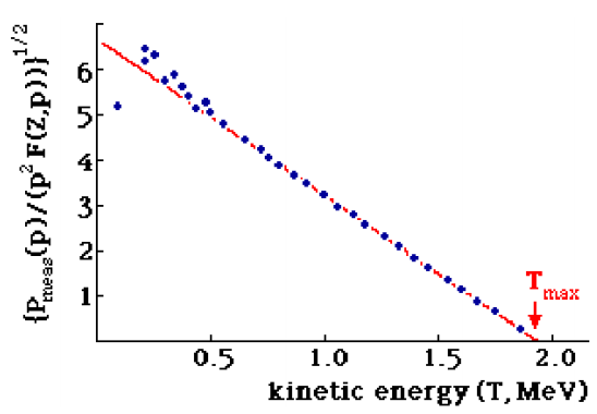
The square root of this quantity is then a linear function in the neutrino kinetic energy, \(Q-T_{e}\):
\[\sqrt{\frac{d W}{d p_{e}} \frac{1}{p_{e}^{2} F(Z, Q)}} \propto Q-T_{e} \nonumber\]
This is the Fermi-Kurie relation. Usually, the Fermi-Kurie plot is used to infer by linear regression the maximum electron energy (or Q) by finding the straight line intercept.