
4.2: Polarisation States and Jones Vectors
( \newcommand{\kernel}{\mathrm{null}\,}\)
We have seen in Chapter 1 that light is an electromagnetic wave which satisfies Maxwell’s equations and the wave equation derived therefrom. Since the electric field is a vector that oscillates in a certain direction, we say that the wave has a certain polarisation. In this chapter we look at the different types of polarisation and how the polarisation of a light beam can be manipulated.
We start with Eqs. (1.6.9) and (1.6.11) which show that the electric field E(r,t) of a plane wave is always perpendicular to the direction of propagation, which is the direction of the wave vector k. Let the wave propagate in the z-direction: k=(00k) Then the electric field vector does not have a z-component and hence the real electric field at z and at time t can be written as E(z,t)=(Axcos(kz−ωt+φx)Aycos(kz−ωt+φy)0). where Ax and Ay are positive amplitudes and φx,φy are the phases of the electric field components. While k and ω are fixed in this case, we can vary Ax,Ay,φx and φy. This degree of freedom is why different states of polarisation exist: the state of polarisation is determined by the ratio of the amplitudes and by the phase difference φy−φx between the two orthogonal components of the light wave. Varying the quantity φy−φx means that we are ’shifting’ Ey(r,t) with respect to Ex(r,t). Consider the electric field in a fixed plane z=0 : (Ex(0,t)Ey(0,t))=(Axcos(−ωt+φx)Aycos(−ωt+φy))=Re{(Ex(0)Ey(0))e−iωt}=Re{(AxeiφxAyeiφy)e−iωt}. The complex vector J=(Ex(0)Ey(0))=(AxeiφxAyeiφy) is called the Jones vector. It is used to characterise the polarisation state. Let us see how, at a fixed position in space, the electric field vector behaves as a function of time for different choices of Ax,Ay and φy−φx.
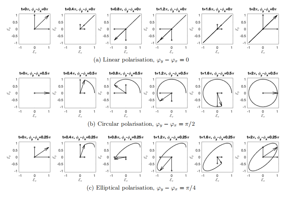
a) Linear polarisation: φy−φx=0 or φy−φx=π. When φy−φx=0 we have J=(AxAy)eiφx Equality of the phases: φy=φx, means that the field components Ex(z,t) and Ey(z,t) are in phase: when Ex(z,t) is large, Ey(z,t) is large, and when Ex(z,t) is small, Ey(z,t) is small. We can write (Ex(0,t)Ey(0,t))=(AxAy)cos(ωt−φx), which shows that for φy−φx=0 the electric field simply oscillates in one direction given by real the vector Axˆx+Ayˆy. See Figure 4.2.1a.
If φy−φx=π we have J=(Ax−Ay)eiφx In this case Ex(z,t) and Ey(z,t) are out of phase and the electric field oscillates in the direction given by the real vector Axˆx−Ayˆy.
b) Circular polarisation: φy−φx=±π/2,Ax=Ay. In this case the Jones vector is: J=(1±i)Axeiφx The field components Ex(z,t) and Ey(z,t) are π/2 radians (90 degrees) out of phase: when Ex(z,t) is large, Ey(z,t) is small, and when Ex(z,t) is small, Ey(z,t) is large. We can write for z=0 and with φx=0 : (Ex(0,t)Ey(0,t))=(Axcos(−ωt)Axcos(−ωt±π/2))=Ax(cos(ωt)±sin(ωt)). The electric field vector moves in a circle. When for an observer looking towards the source, the electric field is rotating anti-clockwise, the polarisation is called left-circularly polarised ( + sign in ( 4.2.9 )), while if the electric vector moves clockwise, the polarisation is called right-circularly polarised (- sign in ( 4.2.9 )).
c) Elliptical polarisation: φy−φx=±π/2,Ax and Ay arbitrary. The Jones vector is: J=(Ax±iAy)eiφx In this case we get instead of ( 4.2.9 ) (again taking φx=0 ): (Ex(0,t)Ey(0,t))=(Axcos(ωt)±Aysin(ωt)). which shows that the electric vector moves along an ellipse with major and minor axes parallel to the x - and y-axis. When the +sign applies, the field is called left-elliptically polarised, otherwise it is called right-elliptically polarised.
d) Elliptical polarisation: φy−φx= anything else, Ax and Ay arbitrary. The Jones vector is now the most general one: J=(AxeiφxAyeiφy) It can be shown that the electric field vector moves always along an ellipse. The exact shape and orientation of this ellipse of course varies with the difference in phase φy−φx and the ratio of the amplitude Ax,Ay and, except when φy−φx=±π/2, the major and minor axis of the ellipse are not parallel to the x - and y-axis. See Figure 4.2.1 c.
Remarks.
1. Frequently the Jones vector is normalised such that|Jx|2+|Jy|2=1. The normalized vector represents of course the same polarisation state as the unnormalised one. In general, multiplying the Jones vector by a complex number does not change the polarisation state. If we multiply for example by eiθ, this has the same result as changing the instant that t=0, hence it does not change the polarisation state. In fact: E(0,t)=Re[eiθJe−iωt]=Re[Je−iω(t−θ/ω)]
2. We will show in section 6.2 that a general time-harmonic electromagnetic field, is a superposition of plane waves with wave vectors of the same length determined by the frequency of the wave but with different directions. An example is the electromagnetic field near the focal plane of a lens. There is then no particular direction of propagation to which the electric field should be perpendicular; in other words, there is no obvious choice for a plane in which the electric field oscillates as function of time. Nevertheless, for every point in space, such a plane exists, but its orientation varies in general with position. Furthermore, the electric field in a certain point moves along an ellipse in the corresponding plane, but the shape of the ellipse and the orientation of its major axis can be arbitrary. We can conclude that in any point of an arbitrary time-harmonic electromagnetic field, the electric (and in fact also the magnetic) field vector prescribes as function of time an ellipse in a certain plane which depends on position. In this chapter we only consider the field and polarisation state of a single plane wave.
KhanAcademy - Polarization of light, linear and circular: Explanation of different polarisation states and their applications.