2.7: Examples
- Page ID
- 8300
\( \newcommand{\vecs}[1]{\overset { \scriptstyle \rightharpoonup} {\mathbf{#1}} } \)
\( \newcommand{\vecd}[1]{\overset{-\!-\!\rightharpoonup}{\vphantom{a}\smash {#1}}} \)
\( \newcommand{\dsum}{\displaystyle\sum\limits} \)
\( \newcommand{\dint}{\displaystyle\int\limits} \)
\( \newcommand{\dlim}{\displaystyle\lim\limits} \)
\( \newcommand{\id}{\mathrm{id}}\) \( \newcommand{\Span}{\mathrm{span}}\)
( \newcommand{\kernel}{\mathrm{null}\,}\) \( \newcommand{\range}{\mathrm{range}\,}\)
\( \newcommand{\RealPart}{\mathrm{Re}}\) \( \newcommand{\ImaginaryPart}{\mathrm{Im}}\)
\( \newcommand{\Argument}{\mathrm{Arg}}\) \( \newcommand{\norm}[1]{\| #1 \|}\)
\( \newcommand{\inner}[2]{\langle #1, #2 \rangle}\)
\( \newcommand{\Span}{\mathrm{span}}\)
\( \newcommand{\id}{\mathrm{id}}\)
\( \newcommand{\Span}{\mathrm{span}}\)
\( \newcommand{\kernel}{\mathrm{null}\,}\)
\( \newcommand{\range}{\mathrm{range}\,}\)
\( \newcommand{\RealPart}{\mathrm{Re}}\)
\( \newcommand{\ImaginaryPart}{\mathrm{Im}}\)
\( \newcommand{\Argument}{\mathrm{Arg}}\)
\( \newcommand{\norm}[1]{\| #1 \|}\)
\( \newcommand{\inner}[2]{\langle #1, #2 \rangle}\)
\( \newcommand{\Span}{\mathrm{span}}\) \( \newcommand{\AA}{\unicode[.8,0]{x212B}}\)
\( \newcommand{\vectorA}[1]{\vec{#1}} % arrow\)
\( \newcommand{\vectorAt}[1]{\vec{\text{#1}}} % arrow\)
\( \newcommand{\vectorB}[1]{\overset { \scriptstyle \rightharpoonup} {\mathbf{#1}} } \)
\( \newcommand{\vectorC}[1]{\textbf{#1}} \)
\( \newcommand{\vectorD}[1]{\overrightarrow{#1}} \)
\( \newcommand{\vectorDt}[1]{\overrightarrow{\text{#1}}} \)
\( \newcommand{\vectE}[1]{\overset{-\!-\!\rightharpoonup}{\vphantom{a}\smash{\mathbf {#1}}}} \)
\( \newcommand{\vecs}[1]{\overset { \scriptstyle \rightharpoonup} {\mathbf{#1}} } \)
\(\newcommand{\longvect}{\overrightarrow}\)
\( \newcommand{\vecd}[1]{\overset{-\!-\!\rightharpoonup}{\vphantom{a}\smash {#1}}} \)
\(\newcommand{\avec}{\mathbf a}\) \(\newcommand{\bvec}{\mathbf b}\) \(\newcommand{\cvec}{\mathbf c}\) \(\newcommand{\dvec}{\mathbf d}\) \(\newcommand{\dtil}{\widetilde{\mathbf d}}\) \(\newcommand{\evec}{\mathbf e}\) \(\newcommand{\fvec}{\mathbf f}\) \(\newcommand{\nvec}{\mathbf n}\) \(\newcommand{\pvec}{\mathbf p}\) \(\newcommand{\qvec}{\mathbf q}\) \(\newcommand{\svec}{\mathbf s}\) \(\newcommand{\tvec}{\mathbf t}\) \(\newcommand{\uvec}{\mathbf u}\) \(\newcommand{\vvec}{\mathbf v}\) \(\newcommand{\wvec}{\mathbf w}\) \(\newcommand{\xvec}{\mathbf x}\) \(\newcommand{\yvec}{\mathbf y}\) \(\newcommand{\zvec}{\mathbf z}\) \(\newcommand{\rvec}{\mathbf r}\) \(\newcommand{\mvec}{\mathbf m}\) \(\newcommand{\zerovec}{\mathbf 0}\) \(\newcommand{\onevec}{\mathbf 1}\) \(\newcommand{\real}{\mathbb R}\) \(\newcommand{\twovec}[2]{\left[\begin{array}{r}#1 \\ #2 \end{array}\right]}\) \(\newcommand{\ctwovec}[2]{\left[\begin{array}{c}#1 \\ #2 \end{array}\right]}\) \(\newcommand{\threevec}[3]{\left[\begin{array}{r}#1 \\ #2 \\ #3 \end{array}\right]}\) \(\newcommand{\cthreevec}[3]{\left[\begin{array}{c}#1 \\ #2 \\ #3 \end{array}\right]}\) \(\newcommand{\fourvec}[4]{\left[\begin{array}{r}#1 \\ #2 \\ #3 \\ #4 \end{array}\right]}\) \(\newcommand{\cfourvec}[4]{\left[\begin{array}{c}#1 \\ #2 \\ #3 \\ #4 \end{array}\right]}\) \(\newcommand{\fivevec}[5]{\left[\begin{array}{r}#1 \\ #2 \\ #3 \\ #4 \\ #5 \\ \end{array}\right]}\) \(\newcommand{\cfivevec}[5]{\left[\begin{array}{c}#1 \\ #2 \\ #3 \\ #4 \\ #5 \\ \end{array}\right]}\) \(\newcommand{\mattwo}[4]{\left[\begin{array}{rr}#1 \amp #2 \\ #3 \amp #4 \\ \end{array}\right]}\) \(\newcommand{\laspan}[1]{\text{Span}\{#1\}}\) \(\newcommand{\bcal}{\cal B}\) \(\newcommand{\ccal}{\cal C}\) \(\newcommand{\scal}{\cal S}\) \(\newcommand{\wcal}{\cal W}\) \(\newcommand{\ecal}{\cal E}\) \(\newcommand{\coords}[2]{\left\{#1\right\}_{#2}}\) \(\newcommand{\gray}[1]{\color{gray}{#1}}\) \(\newcommand{\lgray}[1]{\color{lightgray}{#1}}\) \(\newcommand{\rank}{\operatorname{rank}}\) \(\newcommand{\row}{\text{Row}}\) \(\newcommand{\col}{\text{Col}}\) \(\renewcommand{\row}{\text{Row}}\) \(\newcommand{\nul}{\text{Nul}}\) \(\newcommand{\var}{\text{Var}}\) \(\newcommand{\corr}{\text{corr}}\) \(\newcommand{\len}[1]{\left|#1\right|}\) \(\newcommand{\bbar}{\overline{\bvec}}\) \(\newcommand{\bhat}{\widehat{\bvec}}\) \(\newcommand{\bperp}{\bvec^\perp}\) \(\newcommand{\xhat}{\widehat{\xvec}}\) \(\newcommand{\vhat}{\widehat{\vvec}}\) \(\newcommand{\uhat}{\widehat{\uvec}}\) \(\newcommand{\what}{\widehat{\wvec}}\) \(\newcommand{\Sighat}{\widehat{\Sigma}}\) \(\newcommand{\lt}{<}\) \(\newcommand{\gt}{>}\) \(\newcommand{\amp}{&}\) \(\definecolor{fillinmathshade}{gray}{0.9}\)Example \(\PageIndex{1}\)
A real object is 15 cm from a converging lens of focal length 25 cm. Where is the image? Describe it.
Light diverges from a real object, so the initial convergence is negative. \(C_1\) = −1/15 cm −1. The power of the converging lens is \(P\) = + 1/25 cm−1. The final convergence is
\( C_2 = -\frac{1}{15}+ \frac{1}{25} = -\frac{2}{75}\)cm −1.
The image is 37.5 cm from the lens. Light is diverging after it leaves the lens. The image is on the same side of the lens as the object is. It is a virtual image. The magnification is \(C_1/C_2 = +2.5\). The image is erect and magnified in size.
Example \(\PageIndex{2}\)
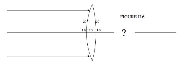
The faces of a biconvex lens have radii of curvature 20 cm and 30 cm, and the refractive index of the glass is 1.5. What is the focal length of the lens?
Refer to Figure II.6.
The initial convergence is zero. The final convergence will be \(1/f\). The power of the first surface is \( \frac{1.5-1.0}{+20}\) cm−1.The power of the second surface is \(\frac{1.0-1.5}{-30}\) cm −1. Note that the radius of curvature of the second surface, when encountered by the light, is negative.
Therefore
\( \frac{1}{f} = \frac{1.5-1.0}{+20}+\frac{1.0-1.5}{-30}.\)
\(f\) = 24 cm.
The lens is a converging lens.
Example \(\PageIndex{3}\)
What is the focal length of this lens, in which I have marked the radii of curvature in cm and the refractive indices?
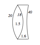
The power, which is the reciprocal of the focal length, is the sum of the powers of the three interfaces:
\(\frac{1}{f} = \frac{1.5-1.0}{20}+ \frac{1.6-1.5}{-18} + \frac{1.0-1.6}{40} = + 0.004\) cm−1. \( \qquad \therefore \, f\) = +225.0 cm.
Example \(\PageIndex{4}\)
Let’s now go straight to the impossibly difficult problem of Section 2.1
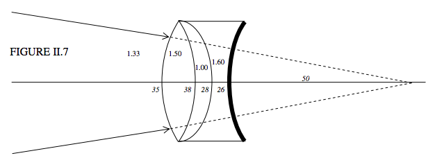
I have marked in the several refractive indices, and, in italics, the radii of curvature and the distance of the virtual object, in cm. Remember that, notwithstanding the drawing, we are assuming that all lenses are thin – that is to say that their thicknesses are negligible compared with other distances.
The system is immersed in water, so the initial convergence is +1.33/50. We are going to find the final convergence. To the initial convergence we are going to add, successively, the powers of the first three refracting interfaces, then the reflecting surface, and then the three refracting surfaces again on the way out. Watch for the refractive indices and the signs of the radii of curvature in each term. The calculation goes like this – as fast as you can write: Final convergence =
\( +\frac{1.33}{50} + \frac{1.50-1.33}{35}+\frac{1.00-1.50}{-38}+\frac{1.60-1.00}{-28}+\frac{-2\times1.60}{+26}+\frac{1.00-1.60}{+28} + \frac{1.50-1.00}{+38}+\frac{1.33-1.50}{-35} \) cm−1.
You can almost double the speed when you realize that the power of a refracting interface is the same whichever way you go (from left to right or from right to left).
We obtain:
Final convergence = −0.103304 cm−1.
Final convergence is refractive index divided by image distance, so the distance of the image from the lens (remember that it’s a thin lens, so don’t ask which part of the lens) is 1.33 ÷ 0.103304, or 12.9 cm.
The light is diverging after it leaves the lens. It is on the same side of the lens as the virtual object is. It is a virtual image. The magnification is initial convergence ÷ final convergence and is therefore −0.257. The image is inverted and diminished in size.
This example perhaps shows the greatest power (pun not intended) of the convergence method – i.e. in dealing with many optical elements one after the other. The is no need for convoluted arguments such as “the real image formed by the first element acts as a virtual object for the second element, and then...”.
Example \(\PageIndex{5}\)
Three observations are performed on a lens in order to determine the radii of curvature of its two surfaces and the refractive index of its glass.
i.) A real object is placed 40 cm to the left of the lens, and a real image is formed 300 cm to the right.
The question doesn’t tell us what sort of a lens it is. Let’s suppose that it is biconvex; we’ll soon find out if it isn’t.
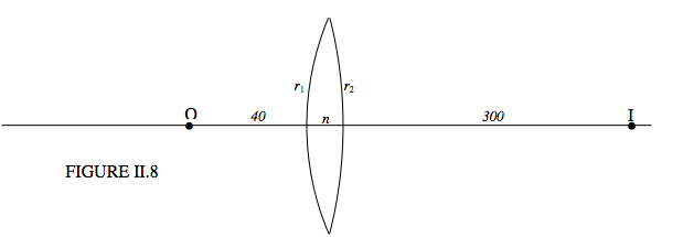
The first experiment tells us:
\( \frac{1}{+300} = -\frac{1}{40} + \frac{n-1}{r_1} + \frac{1-n}{-r_2}. \)
That is
\[(n-1) \left( \frac{1}{r_1} + \frac{1}{r_2}\right) = 0.0283 \text{cm}^{-1} \label{eq:2.7.1} \]
ii.) The lens is floated on the surface of mercury, \(r_1\)-side up. A real object is placed 60 cm above it, and a real image is formed 50 cm above it.
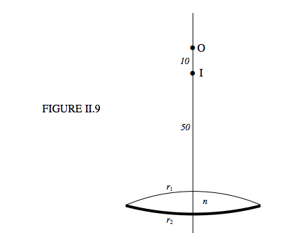
The second experiment tells us:
\( +\frac{1}{50} = -\frac{1}{60}+\frac{n-1}{r_1}+\frac{-2n}{-r_2}+ \frac{1-n}{-r_1} \).
That is:
\[\frac{n-1}{r_1}+\frac{n}{r_2} = 0.0183. \label{eq:2.7.2} \]
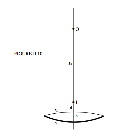
iii.) The lens is floated on the surface of mercury, \(r_2\)-side up. A real object is placed 60 cm above it, and a real image is formed 6 cm above it. (Figure II.10.)
It is necessary to remind ourselves that, the drawing notwithstanding, the lens is thin and all angles are small. The third experiment tells us:
\( +\frac{1}{6} = -\frac{1}{6-}+\frac{n-1}{r_2}+\frac{-2n}{-r_1}+\frac{1-n}{-r_2}. \)
That is
\[ \frac{n-1}{r_2} + \frac{n}{r_1} = 0.0916. \label{eq:2.7.3} \]
Thus we have three nonlinear equations to solve for the three unknowns. Three nonlinear equations have been known to make grown men tremble in their shoes, but fortunately, these three are trivial to solve. It might help to let \(s = 1/r_1\) and \(t = r_2\), when the equations become
\[(n-1)(s+t) = 0.0283. \label{eq:2.7.4} \]
\[ (n-1)s+nt= 0.0183. \label{eq:2.7.5} \]
\[ (n-1)t+ns = 0.0916. \label{eq:2.7.6} \]
One soon arrives at: \(\underline{n = 1.53, \, r_1 = 15.8\space \text{cm},\space r_2 = −100.0 \, \text{cm}}\).
Our assumption that the lens is biconvex was wrong. The second surface is the other way round, and the lens is a meniscus converging lens.
Exercise \(\PageIndex{1}\)
A converging lens forms a real image of a real object. Show that the least distance between real object and real image is \(4f\), and that the magnification is then −1. Remember this when you are trying to show slides in your living room, and you can’t seem to focus the projector on the screen.
Exercise \(\PageIndex{2}\)
A screen is at a fixed distance from a real object. A converging lens is placed between object and screen so as to throw a magnified inverted real image on the screen. The lens is then moved towards the screen, and, after it has moved a distance \(d\), it is seen to throw another real, inverted image on the screen, but this time diminished. Show that, if the distance between object and screen is \(w\), the focal length of the lens is
\( f= \frac{w^2-d^2}{4w}\)
Exercise \(\PageIndex{3}\)
A beetle on the axis of a converging lens and at a distance greater than \(2f\) from it runs towards the lens at a speed \(v\). Show that its real image moves at a speed \(m^2 v\), where \(m\) is the transverse magnification. In which direction does the image move – towards or away from the lens?
Exercise \(\PageIndex{4}\)
Two media of refractive indices \(n_1\) and \(n_2\) are separated by a spherical refractive interface or by a lens – it doesn’t matter which. An object of length \(\Delta p\) lies along the axis in the \(n_1\) side. As a result, the length of the image is \(\Delta q\). The ratio \(\Delta q/ \Delta p \) is called the longitudinal magnification. Show that
\( m_\text{long} = \frac{n_2}{n_1}m^2_\text{lat}\).
Exercise \(\PageIndex{5}\)
When a converging lens is placed in water (refractive index = \(\frac{3}{4}\) ) its focal length is twice what it is when it is in air. What is the refractive index of the glass of which the lens is made?


