2.1: Waves in a Stretched String
- Page ID
- 7356
\( \newcommand{\vecs}[1]{\overset { \scriptstyle \rightharpoonup} {\mathbf{#1}} } \)
\( \newcommand{\vecd}[1]{\overset{-\!-\!\rightharpoonup}{\vphantom{a}\smash {#1}}} \)
\( \newcommand{\id}{\mathrm{id}}\) \( \newcommand{\Span}{\mathrm{span}}\)
( \newcommand{\kernel}{\mathrm{null}\,}\) \( \newcommand{\range}{\mathrm{range}\,}\)
\( \newcommand{\RealPart}{\mathrm{Re}}\) \( \newcommand{\ImaginaryPart}{\mathrm{Im}}\)
\( \newcommand{\Argument}{\mathrm{Arg}}\) \( \newcommand{\norm}[1]{\| #1 \|}\)
\( \newcommand{\inner}[2]{\langle #1, #2 \rangle}\)
\( \newcommand{\Span}{\mathrm{span}}\)
\( \newcommand{\id}{\mathrm{id}}\)
\( \newcommand{\Span}{\mathrm{span}}\)
\( \newcommand{\kernel}{\mathrm{null}\,}\)
\( \newcommand{\range}{\mathrm{range}\,}\)
\( \newcommand{\RealPart}{\mathrm{Re}}\)
\( \newcommand{\ImaginaryPart}{\mathrm{Im}}\)
\( \newcommand{\Argument}{\mathrm{Arg}}\)
\( \newcommand{\norm}[1]{\| #1 \|}\)
\( \newcommand{\inner}[2]{\langle #1, #2 \rangle}\)
\( \newcommand{\Span}{\mathrm{span}}\) \( \newcommand{\AA}{\unicode[.8,0]{x212B}}\)
\( \newcommand{\vectorA}[1]{\vec{#1}} % arrow\)
\( \newcommand{\vectorAt}[1]{\vec{\text{#1}}} % arrow\)
\( \newcommand{\vectorB}[1]{\overset { \scriptstyle \rightharpoonup} {\mathbf{#1}} } \)
\( \newcommand{\vectorC}[1]{\textbf{#1}} \)
\( \newcommand{\vectorD}[1]{\overrightarrow{#1}} \)
\( \newcommand{\vectorDt}[1]{\overrightarrow{\text{#1}}} \)
\( \newcommand{\vectE}[1]{\overset{-\!-\!\rightharpoonup}{\vphantom{a}\smash{\mathbf {#1}}}} \)
\( \newcommand{\vecs}[1]{\overset { \scriptstyle \rightharpoonup} {\mathbf{#1}} } \)
\( \newcommand{\vecd}[1]{\overset{-\!-\!\rightharpoonup}{\vphantom{a}\smash {#1}}} \)
\(\newcommand{\avec}{\mathbf a}\) \(\newcommand{\bvec}{\mathbf b}\) \(\newcommand{\cvec}{\mathbf c}\) \(\newcommand{\dvec}{\mathbf d}\) \(\newcommand{\dtil}{\widetilde{\mathbf d}}\) \(\newcommand{\evec}{\mathbf e}\) \(\newcommand{\fvec}{\mathbf f}\) \(\newcommand{\nvec}{\mathbf n}\) \(\newcommand{\pvec}{\mathbf p}\) \(\newcommand{\qvec}{\mathbf q}\) \(\newcommand{\svec}{\mathbf s}\) \(\newcommand{\tvec}{\mathbf t}\) \(\newcommand{\uvec}{\mathbf u}\) \(\newcommand{\vvec}{\mathbf v}\) \(\newcommand{\wvec}{\mathbf w}\) \(\newcommand{\xvec}{\mathbf x}\) \(\newcommand{\yvec}{\mathbf y}\) \(\newcommand{\zvec}{\mathbf z}\) \(\newcommand{\rvec}{\mathbf r}\) \(\newcommand{\mvec}{\mathbf m}\) \(\newcommand{\zerovec}{\mathbf 0}\) \(\newcommand{\onevec}{\mathbf 1}\) \(\newcommand{\real}{\mathbb R}\) \(\newcommand{\twovec}[2]{\left[\begin{array}{r}#1 \\ #2 \end{array}\right]}\) \(\newcommand{\ctwovec}[2]{\left[\begin{array}{c}#1 \\ #2 \end{array}\right]}\) \(\newcommand{\threevec}[3]{\left[\begin{array}{r}#1 \\ #2 \\ #3 \end{array}\right]}\) \(\newcommand{\cthreevec}[3]{\left[\begin{array}{c}#1 \\ #2 \\ #3 \end{array}\right]}\) \(\newcommand{\fourvec}[4]{\left[\begin{array}{r}#1 \\ #2 \\ #3 \\ #4 \end{array}\right]}\) \(\newcommand{\cfourvec}[4]{\left[\begin{array}{c}#1 \\ #2 \\ #3 \\ #4 \end{array}\right]}\) \(\newcommand{\fivevec}[5]{\left[\begin{array}{r}#1 \\ #2 \\ #3 \\ #4 \\ #5 \\ \end{array}\right]}\) \(\newcommand{\cfivevec}[5]{\left[\begin{array}{c}#1 \\ #2 \\ #3 \\ #4 \\ #5 \\ \end{array}\right]}\) \(\newcommand{\mattwo}[4]{\left[\begin{array}{rr}#1 \amp #2 \\ #3 \amp #4 \\ \end{array}\right]}\) \(\newcommand{\laspan}[1]{\text{Span}\{#1\}}\) \(\newcommand{\bcal}{\cal B}\) \(\newcommand{\ccal}{\cal C}\) \(\newcommand{\scal}{\cal S}\) \(\newcommand{\wcal}{\cal W}\) \(\newcommand{\ecal}{\cal E}\) \(\newcommand{\coords}[2]{\left\{#1\right\}_{#2}}\) \(\newcommand{\gray}[1]{\color{gray}{#1}}\) \(\newcommand{\lgray}[1]{\color{lightgray}{#1}}\) \(\newcommand{\rank}{\operatorname{rank}}\) \(\newcommand{\row}{\text{Row}}\) \(\newcommand{\col}{\text{Col}}\) \(\renewcommand{\row}{\text{Row}}\) \(\newcommand{\nul}{\text{Nul}}\) \(\newcommand{\var}{\text{Var}}\) \(\newcommand{\corr}{\text{corr}}\) \(\newcommand{\len}[1]{\left|#1\right|}\) \(\newcommand{\bbar}{\overline{\bvec}}\) \(\newcommand{\bhat}{\widehat{\bvec}}\) \(\newcommand{\bperp}{\bvec^\perp}\) \(\newcommand{\xhat}{\widehat{\xvec}}\) \(\newcommand{\vhat}{\widehat{\vvec}}\) \(\newcommand{\uhat}{\widehat{\uvec}}\) \(\newcommand{\what}{\widehat{\wvec}}\) \(\newcommand{\Sighat}{\widehat{\Sigma}}\) \(\newcommand{\lt}{<}\) \(\newcommand{\gt}{>}\) \(\newcommand{\amp}{&}\) \(\definecolor{fillinmathshade}{gray}{0.9}\)Before discussing the reflection of light, it will be useful to discuss the following problem. Consider two ropes, one thin and one thick, connected together, and a sinusoidal wave moving from left to right along the ropes:
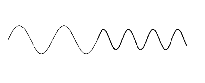
The speed \(c\) of waves in a rope under tension is \(c =\sqrt{F/\mu}\), where \(F\) is the tension, and \(\mu\) is the mass per unit length, so the speed and the wavelength are less in the thicker rope. We’ll call the speed in the left hand rope \(c_1\) and the speed in the right hand rope \(c_2\). At the boundary \((x = 0)\), some of the wave is transmitted, and some is reflected. ( I haven’t drawn the reflected part in the drawing). We wish to find how much is transmitted and how much is reflected. I’ll call the amplitudes of the incident, transmitted and reflected waves 1, \(T\) and \(R\) respectively, and I’ll suppose that the wave is a sinusoidal wave of angular frequency \(\omega\). The equations to the incident, transmitted and reflected waves are as follows:
\[y = \cos \omega \left(t - \dfrac{x}{c_1}\right)\]
\[y = T \cos \omega \left(t - \dfrac{x}{c_2}\right)\]
\[y =R \cos \omega \left(t + \dfrac{x}{c_1}\right)\]
To the right of the boundary, the displacement as a function of \(x\) and \(t\) is
\[y = T \cos \omega \left(t - \dfrac{x}{c_2}\right)\]
and to the left of the boundary the displacement is
\[y = \cos \omega \left(t - \dfrac{x}{c_1}\right) +R \cos \omega \left(t + \dfrac{x}{c_1}\right)\]
At the boundary \((x = 0)\), unless the rope breaks these two displacements must be equal, and therefore
\[ T = 1 + R. \label{eq:2.1} \]
The \(x\)-derivatives (i.e. the slopes) of the ropes are:
To the right of the boundary
\[\dfrac{\partial y}{\partial x}=\dfrac{T}{c_2}\sin\omega\left(t-\dfrac{x}{c_1}\right).\]
and to the left of the boundary
\[\dfrac{\partial y}{\partial x}=\dfrac{A}{c_1}\sin\omega\left(t-\dfrac{x}{c_1}\right) - \dfrac{AR}{c_1}\sin \omega \left(t+\dfrac{x}{c_1}\right).\]
Unless there is a kink in the rope at the boundary, these are equal at \(x = 0\), and therefore
\[ \dfrac{T}{c_2} = \dfrac{1}{c_1} - \dfrac{R}{c_1}. \label{eq:2.2} \]
Combining these with Equation \ref{eq:2.1}, we obtain
\[T = \dfrac{2c_2}{c_2+c_1} \, \text{and} \, R = \dfrac{c_2-c_1}{c_2+c_1}. \label{eq:2.3} \]
We see that if \( c_2 < c_1 \), \(R\) is negative; that is, there is a phase change at reflection. If \(c_2 = c_1\) (i.e. if there is only one sort of rope) there is no reflection (because there is no boundary!).
In the above analysis, we considered a simple sine wave. However, any function, even a nonperiodic function, can be represented by a sum (perhaps an infinite sum) of sinusoidal waves, so the same result will be obtained for any function.
One hopes that energy is conserved, so let’s see. The energy in a wave is proportional to the square of its amplitude and, in the case of a vibrating rope, to the mass per unit length. And the rate of transmission of energy is equal to this times the speed. Thus the rate of transmission of energy is proportional to \(A^2 \mu lc \). However, \(c = \sqrt{F / \mu} \), so that the power is proportional to \(A^2 / c\). Thus the incident, transmitted and reflected powers are in the ratio
\[ 1: \dfrac{4c_1c_2}{(c_1+c_2)^2} : \dfrac{(c_1-c_2)^2}{(c_1+c_2)^2}. \label{eq:2.4} \]
We see that the sum of the transmitted and reflected powers is equal to the incident power, and all’s well with the world.