
4.1: Polarized Light and the Stokes Parameters


- Last updated
- Mar 5, 2022
- Save as PDF

( \newcommand{\kernel}{\mathrm{null}\,}\)
Suppose that we wish to characterize a beam of parallel monochromatic light. A description of it should include the following.
* Its wavelength or frequency. Its wavelength depends upon the refractive index of the material in which it is travelling, whereas its frequency does not. Therefore, if the wavelength is given, the medium must be specified. It may not always be realized, but most tables of wavelengths of spectrum lines in the visible region of the spectrum are given for air and not for a vacuum. [Actually for something called “Standard Air” - details of which may be found in http://orca.phys.uvic.ca/~tatum/stellatm/atm7.pdf ] Specifying the frequency rather than the wavelength removes possible ambiguity. Spectroscopists often quote the wavenumber in vacuo, which is the reciprocal of the vacuum wavelength.
* Its flux density in W m−2. This is related to the electric field strength of the electromagnetic wave, in a manner that will be discussed later in the chapter.
* Its state of polarization. In this chapter, polarized light will in general be taken to mean elliptically polarized light, which includes circularly and linearly (plane) polarized light as special cases. The state of polarization can be described by specifying
* the eccentricity of the polarization ellipse
* the orientation of the polarization ellipse
* the chirality (handedness) of the polarization ellipse
* whether the polarization is total or partial, and, if partial, the degree of polarization.
Up to and including Equation (A15) (page 8) we shall assume that the polarization is total. We shall look at partial polarization after that.
Polarized light is generally described by supposing that, at some point in space, the tip of the vector that represents the strength of the electric field describes a Lissajous ellipse (Figure IV.1).
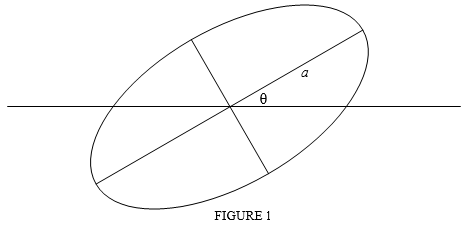
In the drawing the semi major axis a represents the greatest value of the electric field strength, in volts per metre, during a cycle, and the semi minor axis b represent the least value of the electric field strength during the cycle. If you prefer, you could use symbols such as Emax and Emin instead of a and b.
In order to describe the ellipse, we need to describe its size, its shape, its orientation and its chirality or handedness (i.e., whether the vector is rotating clockwise or counterclockwise).
The natural way of doing this is to give the length a of the semi major axis (in volts per metre), the eccentricity of the (e = √1−b2a2) , the angle θ that the major axis makes with the horizontal, and perhaps one of the words "clockwise" or "counterclockwise". It will be necessary, however, to make clear whether you, the observer, are looking towards the source of light, or are looking in the direction of travel of the light. Not everyone uses the same convention in this matter, and the onus is on the writer to make clear which convention he or she is using. In this chapter I shall assume that we are looking towards the source of the light. In Figure IV.1, I have drawn the ellipse with ba = 12 (e = √32 = 0.8660) and θ = 30∘.
[Since I wrote the above paragraph, I received in December 2015 a memorandum from the International Astronomical Union stating that there has long been an IAU convention that position angle is to be reckoned positive in the counterclockwise direction for an observer looking towards the source of light. This is in fact the convention that I use in these notes. The IAU memorandum, however, pointed out that some scientists who investigate the polarization of the Cosmic Background Radiation have been using the opposite convention, and consequently the IAU reiterates its recommendation that all astronomers, including those working on the CBR, use the above convention. This is a good example of what I meant in the previous paragraph. I would emphasize that, even although there is an IAU convention - one which I strongly support - it is incumbent upon YOU, to make certain, if you wish your readers to understand you, to make it unambiguously clear, whenever you write about polarization, as to what convention you are using. And don’t just say “the IAU convention”. Say that angles are reckoned positive if increasing counterclockwise when you are facing towards the source of light. I hope that referees and editors will enforce this!]
We noted above that the flux density of the beam is related to the electric field strength of the electromagnetic wave. In this paragraph and the next we explore this relation. Suppose, for ) example, that the light is plane polarized, and that the maximum value of the electric field is ˆE volts. Its mean square value during a cycle is ¯E 2 = 12ˆE 2. The energy per unit volume is 12 ϵ ¯E 2 = 14 ϵ ˆE 2 J m−3, where ϵ is the permittivity of the medium in which the radiation is travelling. If it is moving at speed v, the flux density of the beam is 14 vϵ ˆE 2 W m−2. The speed of an electromagnetic wave in a medium of permittivity ϵ and permeability μ is given by v = 1√ϵμ, so this expression becomes 14√ϵμˆE 2 = ˆE 24Z, where Z = √μϵ is the impedance (in the sense used in electromagnetic theory) of the medium. For most transparent media, μ is very close to μ0. the permeability of free space. This is not the case for the permittivity, which usually ranges from 1 up to a few tens of times ϵ0. For a vacuum, the impedance has a value of about 377Ω.
If the light is elliptically polarized, the expression for the flux density will be a2 + b24Z, where a and b are the electric fields described in earlier paragraphs. That the ˆE 2 for plane polarized light can be replaced by a2 + b2 for elliptically polarized light should become apparent later while discussing the director circle property of an ellipse.
While these parameters may be the obvious ones to use in describing the state of polarization, the fact is that none of them is directly measurable. What we can measure relatively easily is the intensity of the light when viewed through a polarizing filter oriented at various angles. What we can measure are four parameters known as the Stokes parameters, which we shall describe shortly. We can measure the Stokes parameters, and it will then be our task to determine from these the eccentricity, orientation and chirality of the polarization ellipse, and the degree of polarization.
Before describing them, a word about notation.
The traditional symbols used to describe the Stokes parameters are IQUV. These may seem somewhat haphazard, so some modern authors prefer a more systematic S1, S2, S3, S4 while some prefer S0, S1, S2, S3. If you use the modern S notation, I would (strongly) recommend S0, S1, S2, S3 over S1, S2, S3, S4. In these notes, however, I shall be old-fashioned and I shall use IQUV , which at least has the advantage of avoiding the ambiguity over the two possible S notations, and you will not have to worry which version I am using.
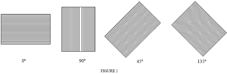
In the figure the lines represent the component of the electric field passed by the filter. The lengths of the long organic molecules embedded within the filter are perpendicular to this transmission direction. Light (i.e. an oscillating electromagnetic field) that is oscillating parallel to the lengths of these molecules is strongly absorbed, because of the highly anisotropic polarizability of these molecules.
Perhaps we can measure the intensity of the light after passage through the filter at each of these angles, and also without the filter, and somehow determine from these measurements the shape and orientation of the polarization ellipse.
The Stokes parameters are named after a nineteenth century British physicist, Sir George Stokes, and may be referred to as Stokes's parameters, Stokes' parameters or the Stokes parameters, but not, of course, as Stoke's parameters.
Let us imagine that we have in our hand a flux meter, and that it can measure the flux density, in W m−2 of our parallel beam of monochromatic light. While we would prefer to use the symbol F for flux density, in fact the flux density of the unobstructed light is the first of the Stokes parameters, for which the traditional symbol is I (and whose modern symbol is S0 or S1, depending on which book you are reading.)
Now let us suppose that we measure the flux density of the light after passage through a polarizing filter oriented at various angles as suggested in Figure IV.2. The second and third Stokes parameters, then, are defined by
Q = F0 − F90
and
U = F45 − F135
Unless you are fortunate or rich, it is unlikely that your little flux meter will accurately measure the flux densities in absolute SI units in W m−2. Therefore those of us of more modest means will just have to be content with dimensionless Stokes parameters - measured in units so that the unobstructed flux density is 1. We define the dimensionless Stokes parameters (for which I use a different font) by
Q = F0 − F90F = QI
U = F45 − F135F = UI
Thus, for the dimensioned Stokes parameters in W m−2 (which we may not easily be able to measure), I use IQUV. For the dimensionless Stokes parameters, I use QUV. (There is no need for a dimensionless I, because it is 1.)
It is possible to determine the eccentricity e and the inclination θ of the polarization ellipse from Q and U. Here I give the relations without derivation. I shall give a derivation in an Appendix to this chapter. For the time being, then, here are the relations:
Q = e2cos2θ2 − e2
U = e2sin2θ2 − e2
Perhaps of more interest are the converses of these:
e2 = 2√Q2 + U21 + √Q2 + U2
tan2θ = UQ
In solving Equation (8) for θ, it is necessary to know the signs of U and Q separately, in order to avoid an ambiguity of quadrant. Provision of the arctan2 function in a calculator or computer greatly facilitates this.
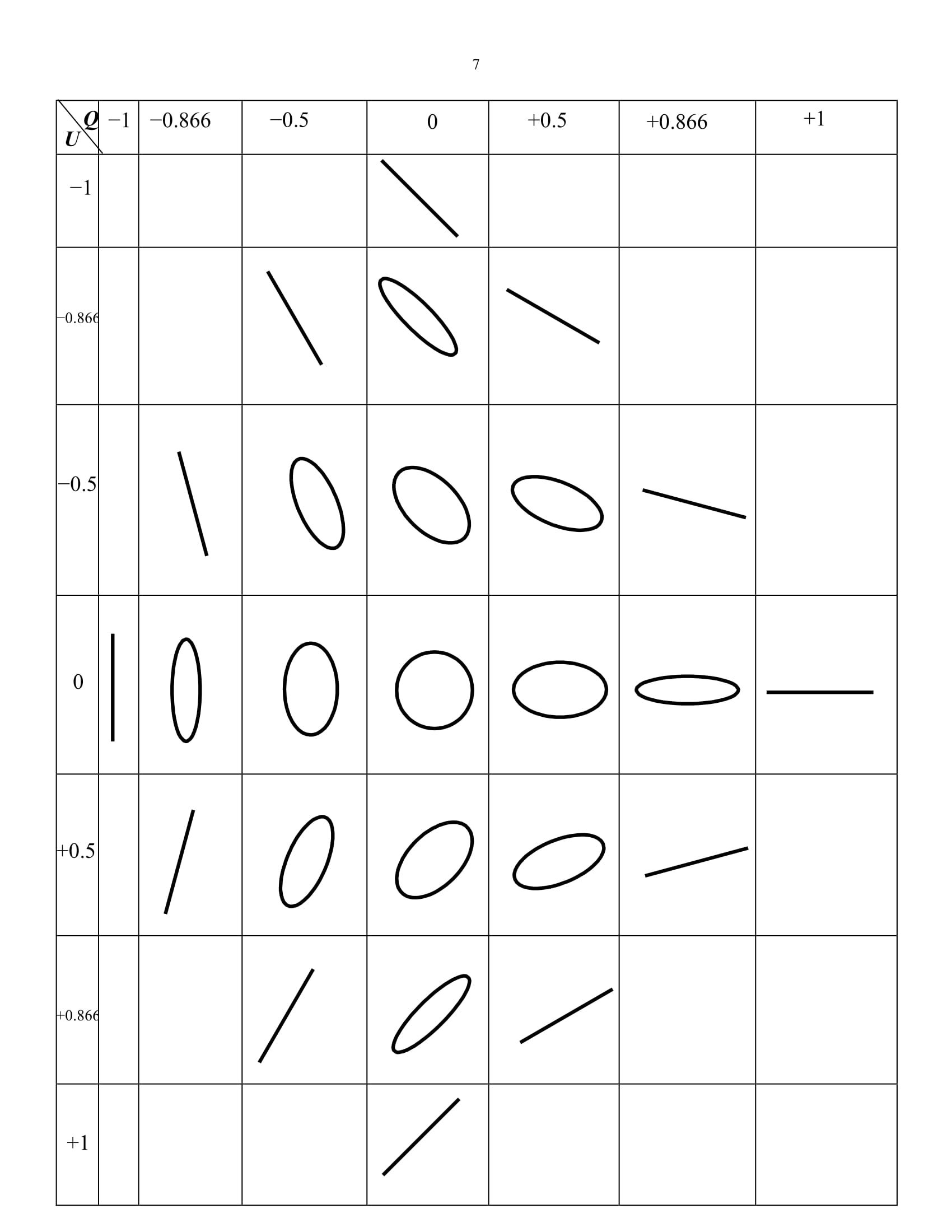
The table below shows a sample of polarization ellipses for various combinations of Q and U. For reasons that will become apparent during the derivation of the formulas in the Appendix, all of the ellipses are drawn such that a2 + b2 is the same for each. This ensures that the flux density is the same for each.
Thus far we have dealt with the Stokes parameters I (related to the flux density of the light), and Q and U (related to the shape and orientation of the polarization ellipse). Now we have to describe the Stokes parameter V, and how it is related to the chirality (handedness) of the ellipse. In this account, when I use the words “clockwise” and “counterclockwise” I shall assume that we are looking towards the source of light.
If we really want to know the polarity, we need to have a good research grant and to be in possession of a filter that passes only circularly polarized light. A linear polarizer in conjunction with a quarter-wave plate will do it. I shall take it that the filter passes only light that is circularly polarized in the clockwise sense. Suppose the flux density after passage through such a filter is FC. The Stokes V parameter is defined as
V = 2FC − I,
or, in dimensionless form,
V = 2FCF −1.
It will be observed that this parameter (like the others) ranges from −1 (if FC=0) to +1 (if FC=1), and hence that negative V implies counterclockwise polarization, and positive V implies clockwise polarization. We shall also show in the Appendix, that (subject to an important condition - see below), V is related to the eccentricity by
V2 = 4(1−e2)(2−e2)2.
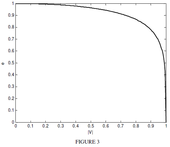
This means that V=0 implies e=1, and hence linear polarization (for which there is no chirality). Also, V2=1 implies e=1, and hence circular polarization. Conversely
e2=2(−1+V2+√1−V2)V2
Thus one can determine both the chirality and the eccentricity (but not θ) from V alone. Figure IV.3 shows the relation between |V| and e.
This redundancy must mean that Q,U and V are not independent, and indeed it will be observed from equations (5), (6) and (11) that
Q2 + U2 + V2 = 1.
In terms of the dimensioned Stokes parameters:
Q2 + U2 + V2 = I2.
In one of the S notations, this would conveniently be
S21+S22+S23=S20.
Just before Equation (11) we referred to an important condition. Equations (11) - (15), and Figure IV.3, are valid only for the case of total elliptical polarization. The case of partial polarization is discussed in what follows. The section on partial polarization should not be thought of as a relatively unimportant afterthought, because most sources of polarized light that one comes across are more likely to be partially polarized rather than totally polarized.
Partial Polarization
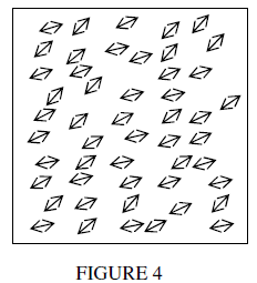
Until this point we have assumed that we have been concerned with a single coherent wave with one well-defined polarization state. In practice, we rarely see this, and we more often have to deal with partially polarized light. Most of us have a fairly good idea of what is meant by light that is partially plane polarized horizontally. We mean that the light is mostly like this:

but there’s also a little bit of this:

But if that were so with two coherent waves, this would result, if they were in phase, in this:
or if they were not in phase, in this:
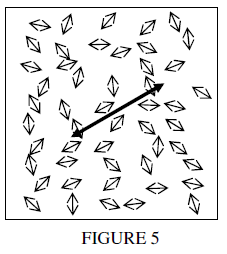
In truth, unless we are looking at a coherent light source, such as a laser, partially polarized light might be more like this:
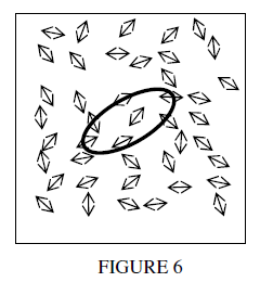
This is partially plane polarized at about an angle of 30º, but it is clearly not totally plane polarized. Partially polarized light can be described as the sum of a totally polarized component plus an unpolarized component. Thus we might describe the situation illustrated above by something like this:
Partially elliptical polarized light might be described by a totally elliptically polarized component, plus an unpolarized component:
If we could somehow separately measure the flux densities of the polarized (p) and unpolarized (u) components, we could define the degree of polarization by
p = FpFp + Fu
If we know that the light is partially plane (linearly) polarized, as in Figure IV.5 (rather than elliptically polarized as in Figure IV.6), we can measure this rather easily. Place the polarizing filter in front of the source, and rotate it until the transmitted flux density goes through a maximum, Fmax. and then through a further 90º until it goes through a minimum, Fmin. This will give you the degree of polarization from.
p = Fmax − FminFmax + Fmin.
and of course it also gives you the polarization angle. This applies, of course, only to light that you know to be partially linearly polarized. It will not do for partially elliptically polarized light.
Recall that
Q = F0 − F90F = QI
and
U = F45 − F135F = UI
If the source is partially plane polarized, each of the measurements F0,F90,F45,F135 includes a total linear or elliptical component, and an unpolarized component. However, the unpolarized component is the same for each of these four measurements. Consequently Q and U describe the “total” component only. Thus all equations up to and including Equation (8), as well as the table illustrating the shape of the ellipse as a function of Q and U, are still valid for the “total” component.
The parameter V, however, was defined in Equations 9 and 10 by
V = 2FC − I,
or, in dimensionless form,
V = 2FCF −1.
FC and F each contain a “total” and an unpolarized component, so that, unlike Q and U, the “total” component is not separated out.
Recall from Equations (13) and (14) that I = √Q2 + U2 + V2 and Q2 + U2 + V2 = 1.
These were derived for totally elliptically (which includes linearly) polarized light. For light that is partially polarized, it applies only to the “total” part, so that, for partially polarized light,
p = √Q2 + U2 + V2.
From Equations (5), (6) and (18) we determine that
p = √V2 + e4(2−e2)2
Thus from the measurements of F0,F90,F45,F135 and their combinations IQUV we have determined, for partially polarized light, the degree of polarization, and the eccentricity, orientation and chirality of the polarization ellipse.
Equation (18) suggests that that the state of polarization of light can be described by a point in QUV space . This concept is described by the Poincaré sphere:
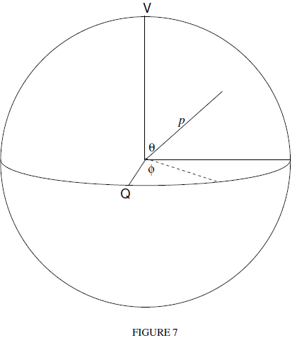
In this context I have often seen the notation 2ψ for ϕ and 2χ for 90º − θ. (The θ here, of course, is not the same as the θ of Figure IV.1.
Let us suppose, to begin with, that we have total polarization, so that p=1. The reader is invited to imagine the shape of the polarization ellipse at any point on the surface of the sphere. Recall in particular that V=0 implies linear polarization, and V=±1 implies circular polarization. Thus anywhere around the equator of the Poincaré represents linear polarization, and at the poles we have circular polarization.
Let us look along the meridian of longitude with ϕ = 0 (U= 0). As we go from the “north pole” to the “south pole”, V goes from +1 (circular) through 0 (linear) to −1 (circular), and Q goes from 0 (circular) through 1 (linear) to 0 (circular). It will be useful (essential) to refer to the table on page 5.
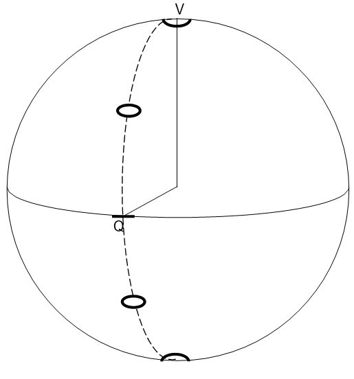
The reader is now invited to think about (while referring to the table on page 5) the situation along the meridian with φ = 90º. And then to try other meridians, eventually covering the sphere with ellipses. This is a little beyond my artistic ability, but I found a very good one by Googling for Poincaré sphere. Choose “Images for poincare sphere”. There are some excellent images there. I particularly like the orange-coloured one from University of Arizona. If you click on it, the sphere rotates, and you can see all round the sphere.
APPENDIX
In the article above I described the Stokes parameters, and I related them to the shape, orientation and chirality of the polarization ellipse, as follows (for total polariazation):
Q = e2cos2θ2−e2U = e2sin2θ2−e2V2 = 4(1−e2)(2−e2)2
In this Appendix, I derive these relations.
Before starting, let us remind ourselves of an established property of an ellipse of semi major and semi minor axes a and b, namely that the locus of the corners of all circumscribing rectangles to an ellipse is a circle, known as the director circle, which is of radius √a2+b2. This is illustrated in Figure A1, in which I have drawn three circumscribing rectangles. The semidiagonals of all the circumscribing rectangles are of the same length, namely √a2+b2. A proof of this theorem is to be found in http://orca.phys.uvic.ca/~tatum/celmechs/celm2.pdf , Section 2.3, or in many books on the properties of the conic sections.
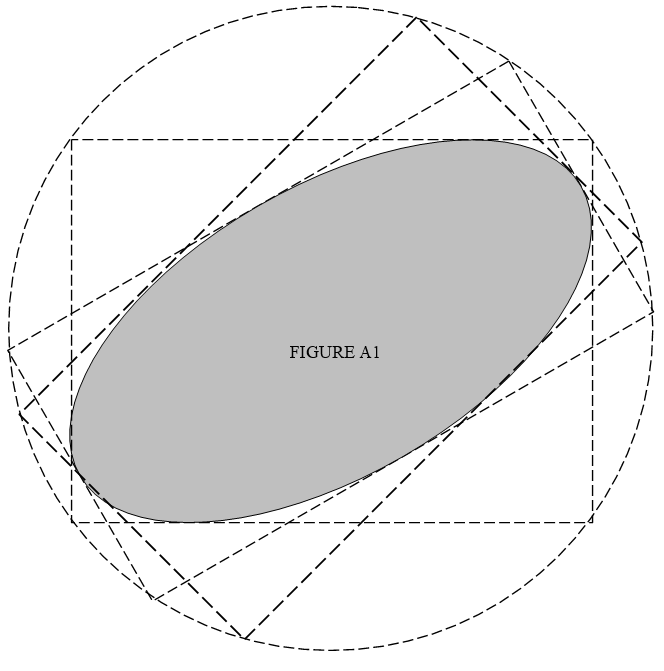
Recall now the meanings of a and b. They are the semi major and semi minor axes of the ellipse, but they are also the greatest and least values of the electric field during a cycle. Recall also that the energy per unit volume of an electric field is proportional to the square of the electric field strength. When the light is observed direct without the intervention of a polarizing filter, the flux density of the light is proportional, then, to a2+b2. That is to say, the Stokes parameter I is proportional to the square of the radius of the director circle.
In what follows, we shall have occasion to refer the polarization ellipse to three rectangular coordinate systems.
i. A coordinate system (x,y), in which the axes of coordinates coincide with the axes of the polarization ellipse.
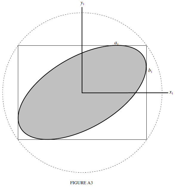
ii. A coordinate system (x1,y1), in which the axes of coordinates are horizontal and vertical - or, to more precise, parallel to the transmission axes of the first two filters illustrated in Figure IV.1.
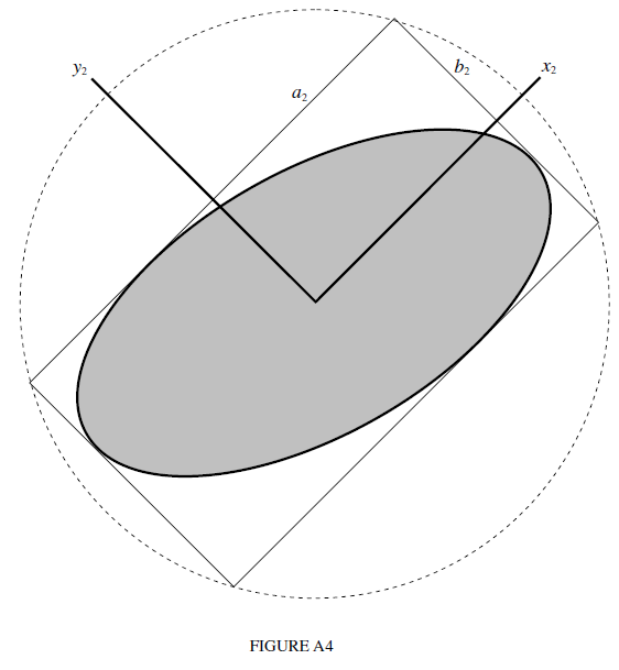
iii. A coordinate system (x2,y2), in which the axes of coordinates are parallel to the transmission axes of the last two filters illustrated in Figure IV.1.
The ellipse referred to these three coordinate systems is shown in Figures A2, A3, A4. In each of these drawings, I have drawn a circumscribing rectangle and the director circle. The flux density of the radiation is proportional to the square of the rectangle diagonal, which is the same in all three drawings, and is equal to the diameter of the director circle, namely 2√a2 + b2.
I have also indicated the lengths a, b, a1, b1, a2, b2 in these drawings. These represent the maximum values of the component of the electric field during a cycle in the directions of the six axes. Indeed, the reader might even prefer an alternative notation:
a = ˆEx
b = ˆEy
a1 = ˆEx1
b1 = ˆEy1
a2 = ˆEx2
b2 = ˆEy2
The first notation is easier for the analysis of the geometry of the ellipse. The second notation reminds us of the physical meaning of the symbols. Indeed the readings of our flux meter are proportional, successively, to ˆEx 2 + ˆEy 2, ˆEx1 2 , ˆEy1 2, ˆEx2 2 , ˆEy2 2, or, in the a,b notation a2 + b2, a21, b21, a22 , b22,. The Stokes parameters I,Q,U are proportional successively to ˆEx 2 + ˆEy 2, ˆEx1 2 − ˆEy1 2, ˆEx2 2 − ˆEy2 2,, or in the a,b notation, a2 + b2, a21 − b21, a22 − b22.
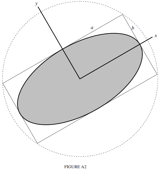
Refer to Figure A2. The equation to the ellipse, referred to this coordinate system, is the familiar
x2a2 + y2b2 = 1,
However, I want to express lengths (electric field strengths) in units such that a2 + b2 =1, and, further, I want to write the equation in terms of the eccentricity e = √1−b2a2. In that case, Equation (A1) becomes
fx2 + gy2 = 1
where
f = 2 − e2 and g = 2−e21−e2.
Now refer to Figure A3. If the major axis of the ellipse makes an angle θ with the horizontal, the coordinate systems are related by
(xy) = (cs−sc)(x1y1),
c=cosθ and s=sinθ
On making use of equations (A2) and (A4), we find that the equation to the ellipse referred to the (x1,y1) coordinate system is
(fc2+gs2)x21−2(g−f)scx1y1+(fs2+gc2)y21=1
We now wish to find a1=ˆEx1 and b1=ˆEy1, the maximum horizontal and vertical components of the electric field. The length a1 can be found as follows. The vertical line x1=a1 intersects this ellipse at values of y1 given by
(fs2+gc2)y21−2(g−f)sca1y1+(fc2+gs2)a21−1=0
But the line x1=a1 is to be a vertical tangent to the ellipse, and therefore the quadratic equation (A6) must have two equal real roots, which tells us, after a little algebra, that
a21=fs2+gc2fg.
A similar analysis starting with the horizontal line y1=b1 reveals that
b21=fc2+gs2fg.
For a check on the correctness of the algebra, it can now be verified that a21+b21=1.
The Stokes Q parameter is a21−b21, and, after some algebra and trigonometric identities, it is found that
Q=a21−b21=e2cos2θ2−e2,
which is one of the relations that we sought.
Now refer to Figure A3. The x2,y2 and x,y coordinate systems are related by
(xy)=(C−SSC)(x2y2),
where
S=sin(45∘−θ)andC=cos(45∘−θ).
On making use of Equations (A2) and (A10), we find that the equation to the ellipse referred to the (x2,y2) coordinate system is
(fC2+gS2)x22+2(g−f)SCx2y2+(fS2+gC2)y22=1
To obtain U, we now proceed in a similar fashion to the analysis of Q. We combine this equation with x2=a2 and put in the condition that the resulting quadratic equation in y2 has two equal real roots, to obtain
a22=fS2+gC2fg
Likewise, by combination with y2=b2, we obtain
b22=fC2+gS2fg
The correctness of the algebra can be checked by verifying that a22+b22=1. Then U, which is a22−b22, can be calculated with some algebra and trigonometry, to be
U=e2sin2θ2−e2.
And this is a good time to remind ourselves of equation (A9)
In our drawings in this chapter, we have taken b=12a,e=√32,θ=30∘ so that Q=0.3,U=0.5196.
Now for the chirality or handedness of the radiation. From measurements of Q and U we have deduced the eccentricity and orientation of the Lissajous ellipse, but we don’t yet know whether the tip of the E-vector is moving clockwise or counterclockwise (as seen when looking towards the source of light). This is what the Stokes V parameter is going to tell us.
It is well known that a Lissajous ellipse can be generated as the resultant of two simple harmonic linear oscillations at right angles to each other. In order to understand the V parameter it is necessary to understand that a Lissajous ellipse can also be generated by two circular motions, of different amplitude, and moving in opposite directions. If the semi major and semi minor axes of the Lissajous ellipse are, respectively, a and b, the radii of the circular components are 12(a+b and 12(a−b (see Figure 11).
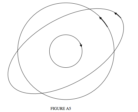
To measure V we place in front of the light source a filter that transmits only circularly polarized light. We’ll suppose that it transmits light that is left-handed (counterclockwise) as seen when looking towards the light source. I.e. it will obstruct the smaller circle of Figure A5 and transmit the large circle.
If the fraction of the flux density passed by the filter is f, the Stokes V parameter is 2f−1.
Examples:
If the light is lefthand circularly polarized, the filter will transmit all of the light. That is, f=1,V=1.
If the light is righthand circularly polarized, the filter will transmit none of the light. That is, f=0,V=−1.
If the light is linearly polarized, the filter will transmit half of the light. (Linearly polarized light can be generated by two equal circles moving in opposite directions.) That is, f=12,V=0.
In Figure A5, b=12. The radius of the small circle (which is obstructed) is 14a and the radius of the large circle (which is transmitted) is 34a. The flux density of the unfiltered light is proportional to a2+b2=54a2. The flux density of the light that is passed is proportional to 98a2. (The flux density, we recall, is proportional to the square of the director circle. The radius of the director circle of the large circle is √(34a)2+(34a2)=√(89a)2. So we have f=0.9,V=0.8.
If we were to reverse all of the arrows in Figure A5, it would be the larger circle that would be blocked and the small circle passed. The flux density of the light that is passed is then proportional to 18a2. So we have f=0.1,V=−0.8.
Thus positive V means that the tip of the E-vector is moving counterclockwise, and negative V means that it is rotating clockwise.
In general, the radius of the large circle is 12(a+b) and the radius of its director circle is 1√2(a+b). If this is the circle that is transmitted, the flux density passed is proportional to 12(a+b)2.
We have, then, f=12(a+b)2a2+b2,V=2aba2+b2. This means, incidentally, that V is proportional to the area of the ellipse. If we take a2+b2=1, then V=2ab. If it is the small circle that is passed, f=12(a−b)2a2+b2,V=−2aba2+b2.
Since the eccentricity of the ellipse is given by e2=1−b2a2, we can express V2 in terms of the eccentricity, thus
V2=4(1−e2)(2−e2)2.
This equation is valid for totally polarized light. For partially polarized light, return to the main text.