
3: Schrödinger and Heisenberg Pictures
- Page ID
- 56457

\( \newcommand{\vecs}[1]{\overset { \scriptstyle \rightharpoonup} {\mathbf{#1}} } \)
\( \newcommand{\vecd}[1]{\overset{-\!-\!\rightharpoonup}{\vphantom{a}\smash {#1}}} \)
\( \newcommand{\dsum}{\displaystyle\sum\limits} \)
\( \newcommand{\dint}{\displaystyle\int\limits} \)
\( \newcommand{\dlim}{\displaystyle\lim\limits} \)
\( \newcommand{\id}{\mathrm{id}}\) \( \newcommand{\Span}{\mathrm{span}}\)
( \newcommand{\kernel}{\mathrm{null}\,}\) \( \newcommand{\range}{\mathrm{range}\,}\)
\( \newcommand{\RealPart}{\mathrm{Re}}\) \( \newcommand{\ImaginaryPart}{\mathrm{Im}}\)
\( \newcommand{\Argument}{\mathrm{Arg}}\) \( \newcommand{\norm}[1]{\| #1 \|}\)
\( \newcommand{\inner}[2]{\langle #1, #2 \rangle}\)
\( \newcommand{\Span}{\mathrm{span}}\)
\( \newcommand{\id}{\mathrm{id}}\)
\( \newcommand{\Span}{\mathrm{span}}\)
\( \newcommand{\kernel}{\mathrm{null}\,}\)
\( \newcommand{\range}{\mathrm{range}\,}\)
\( \newcommand{\RealPart}{\mathrm{Re}}\)
\( \newcommand{\ImaginaryPart}{\mathrm{Im}}\)
\( \newcommand{\Argument}{\mathrm{Arg}}\)
\( \newcommand{\norm}[1]{\| #1 \|}\)
\( \newcommand{\inner}[2]{\langle #1, #2 \rangle}\)
\( \newcommand{\Span}{\mathrm{span}}\) \( \newcommand{\AA}{\unicode[.8,0]{x212B}}\)
\( \newcommand{\vectorA}[1]{\vec{#1}} % arrow\)
\( \newcommand{\vectorAt}[1]{\vec{\text{#1}}} % arrow\)
\( \newcommand{\vectorB}[1]{\overset { \scriptstyle \rightharpoonup} {\mathbf{#1}} } \)
\( \newcommand{\vectorC}[1]{\textbf{#1}} \)
\( \newcommand{\vectorD}[1]{\overrightarrow{#1}} \)
\( \newcommand{\vectorDt}[1]{\overrightarrow{\text{#1}}} \)
\( \newcommand{\vectE}[1]{\overset{-\!-\!\rightharpoonup}{\vphantom{a}\smash{\mathbf {#1}}}} \)
\( \newcommand{\vecs}[1]{\overset { \scriptstyle \rightharpoonup} {\mathbf{#1}} } \)
\(\newcommand{\longvect}{\overrightarrow}\)
\( \newcommand{\vecd}[1]{\overset{-\!-\!\rightharpoonup}{\vphantom{a}\smash {#1}}} \)
\(\newcommand{\avec}{\mathbf a}\) \(\newcommand{\bvec}{\mathbf b}\) \(\newcommand{\cvec}{\mathbf c}\) \(\newcommand{\dvec}{\mathbf d}\) \(\newcommand{\dtil}{\widetilde{\mathbf d}}\) \(\newcommand{\evec}{\mathbf e}\) \(\newcommand{\fvec}{\mathbf f}\) \(\newcommand{\nvec}{\mathbf n}\) \(\newcommand{\pvec}{\mathbf p}\) \(\newcommand{\qvec}{\mathbf q}\) \(\newcommand{\svec}{\mathbf s}\) \(\newcommand{\tvec}{\mathbf t}\) \(\newcommand{\uvec}{\mathbf u}\) \(\newcommand{\vvec}{\mathbf v}\) \(\newcommand{\wvec}{\mathbf w}\) \(\newcommand{\xvec}{\mathbf x}\) \(\newcommand{\yvec}{\mathbf y}\) \(\newcommand{\zvec}{\mathbf z}\) \(\newcommand{\rvec}{\mathbf r}\) \(\newcommand{\mvec}{\mathbf m}\) \(\newcommand{\zerovec}{\mathbf 0}\) \(\newcommand{\onevec}{\mathbf 1}\) \(\newcommand{\real}{\mathbb R}\) \(\newcommand{\twovec}[2]{\left[\begin{array}{r}#1 \\ #2 \end{array}\right]}\) \(\newcommand{\ctwovec}[2]{\left[\begin{array}{c}#1 \\ #2 \end{array}\right]}\) \(\newcommand{\threevec}[3]{\left[\begin{array}{r}#1 \\ #2 \\ #3 \end{array}\right]}\) \(\newcommand{\cthreevec}[3]{\left[\begin{array}{c}#1 \\ #2 \\ #3 \end{array}\right]}\) \(\newcommand{\fourvec}[4]{\left[\begin{array}{r}#1 \\ #2 \\ #3 \\ #4 \end{array}\right]}\) \(\newcommand{\cfourvec}[4]{\left[\begin{array}{c}#1 \\ #2 \\ #3 \\ #4 \end{array}\right]}\) \(\newcommand{\fivevec}[5]{\left[\begin{array}{r}#1 \\ #2 \\ #3 \\ #4 \\ #5 \\ \end{array}\right]}\) \(\newcommand{\cfivevec}[5]{\left[\begin{array}{c}#1 \\ #2 \\ #3 \\ #4 \\ #5 \\ \end{array}\right]}\) \(\newcommand{\mattwo}[4]{\left[\begin{array}{rr}#1 \amp #2 \\ #3 \amp #4 \\ \end{array}\right]}\) \(\newcommand{\laspan}[1]{\text{Span}\{#1\}}\) \(\newcommand{\bcal}{\cal B}\) \(\newcommand{\ccal}{\cal C}\) \(\newcommand{\scal}{\cal S}\) \(\newcommand{\wcal}{\cal W}\) \(\newcommand{\ecal}{\cal E}\) \(\newcommand{\coords}[2]{\left\{#1\right\}_{#2}}\) \(\newcommand{\gray}[1]{\color{gray}{#1}}\) \(\newcommand{\lgray}[1]{\color{lightgray}{#1}}\) \(\newcommand{\rank}{\operatorname{rank}}\) \(\newcommand{\row}{\text{Row}}\) \(\newcommand{\col}{\text{Col}}\) \(\renewcommand{\row}{\text{Row}}\) \(\newcommand{\nul}{\text{Nul}}\) \(\newcommand{\var}{\text{Var}}\) \(\newcommand{\corr}{\text{corr}}\) \(\newcommand{\len}[1]{\left|#1\right|}\) \(\newcommand{\bbar}{\overline{\bvec}}\) \(\newcommand{\bhat}{\widehat{\bvec}}\) \(\newcommand{\bperp}{\bvec^\perp}\) \(\newcommand{\xhat}{\widehat{\xvec}}\) \(\newcommand{\vhat}{\widehat{\vvec}}\) \(\newcommand{\uhat}{\widehat{\uvec}}\) \(\newcommand{\what}{\widehat{\wvec}}\) \(\newcommand{\Sighat}{\widehat{\Sigma}}\) \(\newcommand{\lt}{<}\) \(\newcommand{\gt}{>}\) \(\newcommand{\amp}{&}\) \(\definecolor{fillinmathshade}{gray}{0.9}\)So far we have assumed that the quantum states \(|\psi(t)\rangle\) describing the system carry the time dependence. However, this is not the only way to keep track of the time evolution. Since all physically observed quantities are expectation values, we can write
\[\begin{aligned}
\langle A\rangle &=\operatorname{Tr}[|\psi(t)\rangle\langle\psi(t)| A]=\operatorname{Tr}\left[U(t)|\psi(0)\rangle\langle\psi(0)| U^{\dagger}(t) A\right] \\
&=\operatorname{Tr}\left[|\psi(0)\rangle\langle\psi(0)| U^{\dagger}(t) A U(t)\right] \quad \text { (cyclic property) } \\
& \equiv \operatorname{Tr}[|\psi(0)\rangle\langle\psi(0)| A(t)],
\end{aligned}\tag{3.1}\]
where we defined the time-varying operator \(A(t)=U^{\dagger}(t) A U(t)\). Clearly, we can keep track of the time evolution in the operators!
- Schrödinger picture: Keep track of the time evolution in the states,
- Heisenberg picture: Keep track of the time evolution in the operators.
We can label the states and operators “\(S\)” and “\(H\)” depending on the picture. For example,
\[\left|\psi_{H}\right\rangle=\left|\psi_{S}(0)\right\rangle \quad \text { and } \quad A_{H}(t)=U^{\dagger}(t) A_{S} U(t)\tag{3.2}\]
The time evolution for states is given by the Schrödinger equation, so we want a corresponding “Heisenberg equation” for the operators. First, we observe that
\[U(t)=\exp \left(-\frac{i}{\hbar} H t\right),\tag{3.3}\]
such that
\[\frac{d}{d t} U(t)=-\frac{i}{\hbar} H U(t)\tag{3.4}\]
Next, we calculate the time derivative of \(\langle A\rangle\):
\[\frac{d}{d t} \operatorname{Tr}\left[\left|\psi_{S}(t)\right\rangle\left\langle\psi_{S}(t)\right| A_{S}\right]=\frac{d}{d t}\left\langle\psi_{S}(t)\left|A_{S}\right| \psi_{S}(t)\right\rangle=\frac{d}{d t}\left\langle\psi_{H}\left|A_{H}(t)\right| \psi_{H}\right\rangle\tag{3.5}\]
The last equation follows from Eq. (3.1). We can now calculate
\[\begin{aligned}
\frac{d}{d t}\left\langle\psi_{S}(t)\left|A_{S}\right| \psi_{S}(t)\right\rangle &=\frac{d}{d t}\left\langle\psi_{S}(0)\left|U^{\dagger}(t) A_{S} U(t)\right| \psi_{S}(0)\right\rangle \\
&=\left\langle\psi_{S}(0)\left|\left[\dot{U}^{\dagger}(t) A_{S} U(t)+U^{\dagger}(t) \dot{A}_{S} U(t)+U^{\dagger}(t) A_{S} \dot{U}(t)\right]\right| \psi_{S}(0)\right\rangle \\
&=\left\langle\psi_{H}\left|\left[\frac{i}{\hbar} H A_{H}(t)-\frac{i}{\hbar} A_{H}(t) H+\frac{\partial A_{H}(t)}{\partial t}\right]\right| \psi_{H}\right\rangle \\
&=-\frac{i}{\hbar}\left\langle\psi_{H}\left|\left[A_{H}(t), H\right]\right| \psi_{H}\right\rangle+\left\langle\psi_{H}\left|\frac{\partial A_{H}(t)}{\partial t}\right| \psi_{H}\right\rangle \\
&=\left\langle\psi_{H}\left|\frac{d A_{H}(t)}{d t}\right| \psi_{H}\right\rangle
\end{aligned}\tag{3.6}\]
Since this must be true for all \(\left|\psi_{H}\right\rangle\), this is an operator identity:
\[\frac{d A_{H}(t)}{d t}=-\frac{i}{\hbar}\left[A_{H}(t), H\right]+\frac{\partial A_{H}(t)}{\partial t}\tag{3.7}\]
This is the Heisenberg equation. Note the difference between the “straight \(d\)” and the “curly \(\partial\)” in the time derivative and the partial time derivative, respectively. The partial derivative deals only with the explicit time dependence of the operator. In many cases (such as position and momentum) this is zero.
We have seen that both the Schrödinger and the Heisenberg equation follows from Von Neumann’s Hilbert space formalism of quantum mechanics. Consequently, we have proved that this formalism properly unifies both Schrödingers wave mechanics, and Heisenberg, Born, and Jordans matrix mechanics.
As an example, consider a qubit with time evolution determined by the Hamiltonian \(H=\frac{1}{2} \hbar \omega Z\), with \(Z=\left(\begin{array}{cc} 1 & 0 \\ 0 & -1 \end{array}\right)\). This may be a spin in a magnetic field, for example, such that \(\omega=-e B / m c\). We want to calculate the time evolution of the operator \(X_{H}(t)\). Since we work in the Heisenberg picture alone, we will omit the subscript \(H\). First, we evaluate the commutator in the Heisenberg equation
\[i \hbar \frac{1}{2} \frac{d X}{d t}=\frac{1}{2}[X, H]=-i \hbar \frac{\omega}{2}Y,\tag{3.8}\]
where we defined \(Y=\left(\begin{array}{cc} 0 & -i \\ i & 0 \end{array}\right)\). So now we must know the time evolution of \(Y\) as well:
\[i \hbar \frac{1}{2} \frac{d Y}{d t}=\frac{1}{2}[Y, H]=i \hbar \frac{\omega}{2} X\tag{3.9}\]
These are two coupled linear equations, which are relatively easy to solve:
\[\dot{X}=-\omega Y \quad \text { and } \quad \dot{Y}=\omega X \quad \text { and } \quad \dot{Z}=0\tag{3.10}\]
We can define two new operators \(S_{\pm}=X \pm i Y\), and obtain
\[\dot{S}_{\pm}=-\omega Y \pm i \omega X=\pm i \omega S_{\pm}.\tag{3.11}\]
Solving these two equations yields \(S_{\pm}(t)=S_{\pm}(0) e^{\pm i \omega t}\), and this leads to
\[\begin{aligned}
X(t) &=\frac{S_{+}(t)+S_{-}(t)}{2}=\frac{S_{+}(0) e^{i \omega t}+S_{-}(0) e^{-i \omega t}}{2} \\
&=\frac{1}{2}\left[X(0) e^{i \omega t}+i Y(0) e^{i \omega t}+X(0) e^{-i \omega t}-i Y(0) e^{-i \omega t}\right] \\
&=X(0) \cos (\omega t)-Y(0) \sin (\omega t) .
\end{aligned}\tag{3.12}\]
You are asked to show that \(Y(t)=Y(0) \cos (\omega t)+X(0) \sin (\omega t)\) in exercise 3.
We now take \(\left|\psi_{H}\right\rangle=|0\rangle\) and \(X(0)=\left(\begin{array}{ll} 0 & 1 \\ 1 & 0 \end{array}\right)\), \(Y(0)=\left(\begin{array}{cc} 0 & -i \\ i & 0 \end{array}\right)\). The expectation value of \(X(t)\) is then readily calculated to be
\[\langle 0|X(t)| 0\rangle=\cos (\omega t)\langle 0|X(0)| 0\rangle-\sin (\omega t)\langle 0|Y(0)| 0\rangle=0\tag{3.13}\]
Alternatively, when \(\left|\psi_{H}\right\rangle=|\pm\rangle\), we find
\[\langle+|X(t)|+\rangle=\cos (\omega t) \quad \text { and } \quad\langle+|Y(t)|+\rangle=\sin (\omega t)\tag{3.14}\]
This is a circular motion in time:
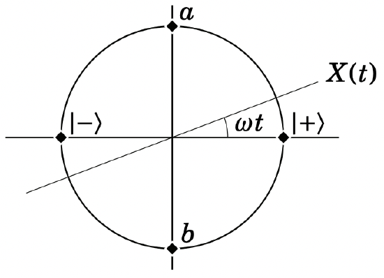
The eigenstate of \(X(\pi / 2)\) is point \(a\), and the eigenstate of \(X(-\pi / 2)\) is point \(b\). Furthermore, \(X(\pm \pi / 2)=\mp Y(0)\), and the states at point \(a\) and \(b\) are therefore the eigenstates of \(Y\):
\[\left|\psi_{a}\right\rangle=\frac{|0\rangle-i|1\rangle}{\sqrt{2}} \quad \text { and } \quad\left|\psi_{b}\right\rangle=\frac{|0\rangle+i|1\rangle}{\sqrt{2}}\tag{3.15}\]
A natural question to ask is where the states \(|0\rangle\) and \(|1\rangle\) fit in this picture. These are the eigenstates of the operator \(Z\), which we used to generate the unitary time evolution. Clearly the states on the circle never become either \(|0\rangle\) or \(|1\rangle\), so we need to add another dimension:
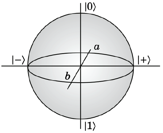
This is called the Bloch sphere, and operators are represented by straight lines through the origin. The axis of rotation for the straight lines that rotate with time is determined by the Hamiltonian. In the above case the Hamiltonian was proportional to \(Z\), which means that the straight lines rotate around the axis through the eigensates of \(Z\), which are \(|0\rangle\) and \(|1\rangle\).
- Show that for the Hamiltonian \(H_{S}=H_{H}\).
- The harmonic oscillator has the energy eigenvalue equation \(H|n\rangle=\hbar \omega\left(n+\frac{1}{2}\right)|n\rangle\).
- The classical solution of the harmonic oscillator is given by
\[|\alpha\rangle=e^{-\frac{1}{2}|\alpha|^{2}} \sum_{n=0}^{\infty} \frac{\alpha^{n}}{\sqrt{n !}}|n\rangle,\tag{3.16}\]
in the limit of \(|\alpha| \gg 1\). Show that \(|\alpha\rangle\) is a properly normalized state for any \(\alpha \in \mathbb{C}\).
- Calculate the time-evolved state \(|\alpha(t)\rangle\).
- We introduce the ladder operators \(\hat{a}|n\rangle=\sqrt{n}|n-1\rangle\) and \(\hat{a}^{\dagger}|n\rangle=\sqrt{n+1}|n+1\rangle\). Show that the number operator defined by \(\hat{n}|n\rangle=n|n\rangle\) can be written as \(\hat{n}=\hat{a}^{\dagger} \hat{a}\).
- Write the coherent state \(|\alpha\rangle\) as a superposition of ladder operators acting on the ground state \(|0\rangle\).
- Note that the ground state is time-independent \((U(t)|0\rangle=|0\rangle)\). Calculate the time evolution of the ladder operators.
- Calculate the position \(\hat{q}=\left(\hat{a}+\hat{a}^{\dagger}\right) / 2\) and momentum \(\hat{p}=-i\left(\hat{a}-\hat{a}^{\dagger}\right) / 2\) of the harmonic oscillator in the Heisenberg picture. Can you identify the classical harmonic motion?
- The classical solution of the harmonic oscillator is given by
- Let \(A\) be an operator given by \(A=a_{0}\mathbb{I}+a_{x} X+a_{y} Y+a_{z} Z\). Calculate the matrix \(A(t)\) given the Hamiltonian \(H=\frac{1}{2} \hbar \omega Z\), and show that \(A\) is Hermitian when the \(a_{\mu}\) are real.
- The interaction picture.
- Let the Hamiltonian of a system be given by \(H=H_{0}+V\), with \(H_{0}=p^{2} / 2 m\). Using \(|\psi(t)\rangle_{I}=U_{0}^{\dagger}(t)|\psi(t)\rangle_{S}\) with \(U_{0}(t)=\exp \left(-i H_{0} t / \hbar\right)\), calculate the time dependence of an operator in the interaction picture \(A_{I}(t)\).
- Defining \(H_{I}(t)=U_{0}^{\dagger}(t) V U_{0}(t)\), show that
\[i \hbar \frac{d}{d t}|\psi(t)\rangle_{I}=H_{I}(t)|\psi(t)\rangle_{I}\tag{3.17}\]
Is \(H_{I}\) identical to \(H_{H}\) and \(H_{S}\)?
- The time operator in quantum mechanics.
- Let \(H|\psi\rangle=E|\psi\rangle\), and assume the existence of a time operator conjugate to \(H\), i.e., \([H, T]=i \hbar\). Show that
\[H e^{i \omega T}|\psi\rangle=(E-\hbar \omega) e^{i \omega T}|\psi\rangle\tag{3.18}\]
- Given that \(\omega \in \mathbb{R}\), calculate the spectrum of \(H\).
- The energy of a system must be bounded from below in order to avoid infinite decay to ever lower energy states. What does this mean for \(T\)?
- Let \(H|\psi\rangle=E|\psi\rangle\), and assume the existence of a time operator conjugate to \(H\), i.e., \([H, T]=i \hbar\). Show that
- Consider a three-level atom with two (degenerate) low-lying states \(|0\rangle\) and \(|1\rangle\) with zero energy, and a high level \(|e\rangle\) (the “excited” state) with energy \(\hbar \omega\). The low levels are coupled to the excited level by optical fields \(\Omega_{0} \cos \omega_{0} t\) and \(\Omega_{1} \cos \omega_{1} t\), respectively.
- Give the (time-dependent) Hamiltonian \(H\) for the system.
- The time dependence in \(H\) is difficult to deal with, so we must transform to the rotating frame via some unitary transformation \(U(t)\). Show that
\(H^{\prime}=U(t) H U^{\dagger}(t)-i \hbar U \frac{d U^{\dagger}}{d t}\)
You can use the Schrödinger equation with \(|\psi\rangle=U^{\dagger}\left|\psi^{\prime}\right\rangle\).
- Calculate \(H^{\prime}\) if \(U(t)\) is given by
\(U(t)=\left(\begin{array}{ccc}
1 & 0 & 0 \\
0 & e^{-i\left(\omega_{0}-\omega_{1}\right) t} & 0 \\
0 & 0 & e^{-i \omega_{0} t}
\end{array}\right)\)Why can we ignore the remaining time dependence in \(H^{\prime}\)? This is called the Rotating Wave Approximation.
- Calculate the \(\lambda=0\) eigenstate of \(H^{\prime}\) in the case where \(\omega_{0}=\omega_{1}\).
- Design a way to bring the atom from the state \(|0\rangle\) to \(|1\rangle\) without ever populating the state \(|e\rangle\).