
7.6: Spherical Harmonics

( \newcommand{\kernel}{\mathrm{null}\,}\)
The simultaneous eigenstates, Yl,m(θ,ϕ), of L2 and Lz are known as the spherical harmonics . Let us investigate their functional form.
We know that L+Yl,l(θ,ϕ)=0, because there is no state for which m has a larger value than +l. Writing Yl,l(θ,ϕ)=Θl,l(θ)eilϕ [see Equations ([e8.34]) and ([e8.38])], and making use of Equation ([e8.28]), we obtain
ℏeiϕ(∂∂θ+icotθ∂∂ϕ)Θl,l(θ)eilϕ=0.
This equation yields dΘl,ldθ−lcotθΘl,l=0. which can easily be solved to give Θl,l∼(sinθ)l. Hence, we conclude that
Likewise, it is easy to demonstrate that
Once we know Yl,l, we can obtain Yl,l−1 by operating on Yl,l with the lowering operator L−. Thus,
Yl,l−1∼L−Yl,l∼e−iϕ(−∂∂θ+icotθ∂∂ϕ)(sinθ)leilϕ,
where use has been made of Equation ([e8.28]). The previous equation yields Yl,l−1∼ei(l−1)ϕ(ddθ+lcotθ)(sinθ)l.
Now, (ddθ+lcotθ)f(θ)≡1(sinθ)lddθ[(sinθ)lf(θ)], where f(θ) is a general function. Hence, we can write
Yl,l−1(θ,ϕ)∼ei(l−1)ϕ(sinθ)l−1(1sinθddθ)(sinθ)2l.
ikewise, we can show that
Yl,−l+1(θ,ϕ)∼L+Yl,−l∼e−i(l−1)ϕ(sinθ)l−1(1sinθddθ)(sinθ)2l.
We can now obtain Yl,l−2 by operating on Yl,l−1 with the lowering operator. We get
Yl,l−2∼L−Yl,l−1∼e−iϕ(−∂∂θ+icotθ∂∂ϕ)ei(l−1)ϕ(sinθ)l−1(1sinθddθ)(sinθ)2l,
which reduces to Yl,l−2∼e−i(l−2)ϕ[ddθ+(l−1)cotθ]1(sinθ)l−1(1sinθddθ)(sinθ)2l. Finally, making use of Equation ([e8.64]), we obtain
Yl,l−2(θ,ϕ)∼ei(l−2)ϕ(sinθ)l−2(1sinθddθ)2(sinθ)2l. Likewise, we can show that
Yl,−l+2(θ,ϕ)∼L+Yl,−l+1∼e−i(l−2)ϕ(sinθ)l−2(1sinθddθ)2(sinθ)2l.
A comparison of Equations ([e8.59]), ([e8.64a]), and ([e8.68]) reveals the general functional form of the spherical harmonics:
Yl,m(θ,ϕ)∼eimϕ(sinθ)m(1sinθddθ)l−m(sinθ)2l.
Here, m is assumed to be non-negative. Making the substitution u=cosθ, we can also write
Yl,m(u,ϕ)∼eimϕ(1−u2)−m/2(ddu)l−m(1−u2)l.
Finally, it is clear from Equations ([e8.60]), ([e8.65]), and ([e8.69]) that
Yl,−m∼Y∗l,m.
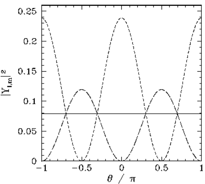
Figure 18: The |Yl,m(θ,ϕ)|2 plotted as a functions of θ. The solid, short-dashed, and long-dashed curves correspond to l,m=0,0, and 1,0, and 1,±1, respectively.
We now need to normalize our spherical harmonic functions so as to ensure that ∮|Yl,m(θ,ϕ)|2dΩ=1. After a great deal of tedious analysis, the normalized spherical harmonic functions are found to take the form Yl,m(θ,ϕ)=(−1)m[2l+14π(l−m)!(l+m)!]1/2Pl,m(cosθ)eimϕ for m≥0, where the Pl,m are known as associated Legendre polynomials , and are written Pl,m(u)=(−1)l+m(l+m)!(l−m)!(1−u2)−m/22ll!(ddu)l−m(1−u2)l for m≥0. Alternatively, Pl,m(u)=(−1)l(1−u2)m/22ll!(ddu)l+m(1−u2)l, for m≥0. The spherical harmonics characterized by m<0 can be calculated from those characterized by m>0 via the identity Yl,−m=(−1)mY∗l,m. The spherical harmonics are orthonormal: that is, ∮Y∗l′,m′Yl,mdΩ=δll′δmm′, and also form a complete set. In other words, any well-behaved function of θ and ϕ can be represented as a superposition of spherical harmonics. Finally, and most importantly, the spherical harmonics are the simultaneous eigenstates of Lz and L2 corresponding to the eigenvalues mℏ and l(l+1)ℏ2, respectively.
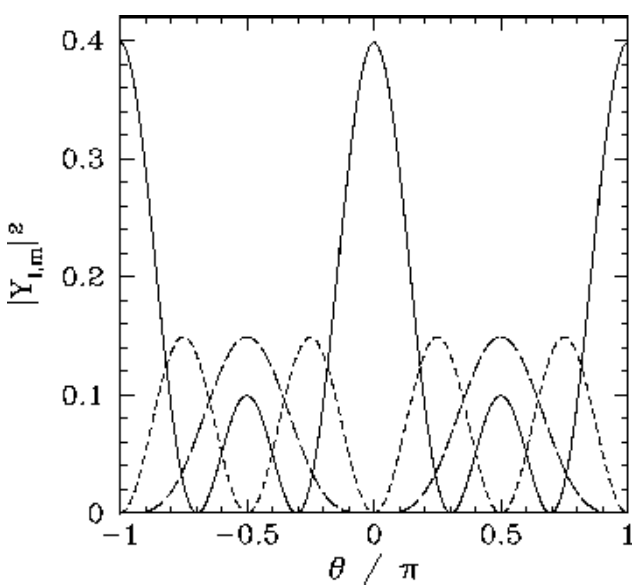
Figure 19: The |Yl,m(θ,ϕ)|2 plotted as a functions of θ. The solid, short-dashed, and long-dashed curves correspond to l,m=2,0, and 2,±1, and 2,±2 respectively.
All of the l=0, l=1, and l=2 spherical harmonics are listed below: Y0,0=1√4π,Y1,0=√34πcosθ,Y1,±1=∓√38πsinθe±iϕ,Y2,0=√516π(3cos2θ−1),Y2,±1=∓√158πsinθcosθe±iϕ,Y2,±2=√1532πsin2θe±2iϕ. The θ variation of these functions is illustrated in Figures [ylm1] and [ylm2].
Contributors and Attributions
Richard Fitzpatrick (Professor of Physics, The University of Texas at Austin)