7.6: Spherical Harmonics

The simultaneous eigenstates, \(Y_{l,m}(\theta,\phi)\), of \(L^2\) and \(L_z\) are known as the spherical harmonics . Let us investigate their functional form.

We know that

\[L_+\,Y_{l,l}(\theta,\phi) = 0, \nonumber \]

because there is no state for which \(m\) has a larger value than \(+l\). Writing

\[Y_{l,l}(\theta,\phi) = {\mit\Theta}_{l,l}(\theta)\,\rm e^{\,{\rm i}\,l\,\phi} \nonumber \]

[see Equations \ref{e8.34} and \ref{e8.38}], and making use of Equation \ref{e8.28}, we obtain

\[\hbar\,\rm e^{\,{\rm i}\,\phi}\left(\frac{\partial}{\partial\theta} + {\rm i}\,\cot\theta\,\frac{\partial}{\partial\phi}\right){\mit\Theta}_{l,l}(\theta)\,\rm e^{\,i\,l\,\phi}=0. \nonumber \]

This equation yields

\[\frac{d{\mit\Theta}_{l,l}}{d\theta} - l\,\cot\theta\,{\mit\Theta}_{l,l} = 0. \nonumber \]

which can easily be solved to give

\[{\mit\Theta}_{l,l}\sim (\sin\theta)^{\,l}. \nonumber \]

Hence, we conclude that

\[ Y_{l,l}(\theta,\phi) \sim (\sin\theta)^{\,l}\,\rm e^{\,{\rm i}\,l\,\phi}. \label{e8.59} \]

Likewise, it is easy to demonstrate that

\[ Y_{l,-l}(\theta,\phi) \sim (\sin\theta)^{\,l}\,\rm e^{-{\rm i}\,l\,\phi}. \label{e8.60} \]

Once we know \(Y_{l,l}\), we can obtain \(Y_{l,l-1}\) by operating on \(Y_{l,l}\) with the lowering operator \(L_-\). Thus,

\[Y_{l,l-1} \sim L_-\,Y_{l,l} \sim \rm e^{-{\rm i}\,\phi}\left(-\frac{\partial}{\partial\theta} + {\rm i}\,\cot\theta\,\frac{\partial}{\partial\phi}\right) (\sin\theta)^{\,l}\,\rm e^{\,{\rm i}\,l\,\phi}, \nonumber \]

where use has been made of Equation \ref{e8.28}. The previous equation yields

\[Y_{l,l-1}\sim \rm e^{\,{\rm i}\,(l-1)\,\phi}\left(\frac{d}{d\theta} +l\,\cot\theta\right)(\sin\theta)^{\,l}. \nonumber \]

Now,

\[ \left(\frac{d}{d\theta}+l\,\cot\theta\right)f(\theta)\equiv \frac{1}{(\sin\theta)^{\,l}}\frac{d}{d\theta}\left[ (\sin\theta)^{\,l}\,f(\theta)\right], \label{e8.64} \]

where \(f(\theta)\) is a general function. Hence, we can write

\[ Y_{l,l-1}(\theta,\phi)\sim \frac{\rm e^{\,{\rm i}\,(l-1)\,\phi}}{(\sin\theta)^{\,l-1}}\left(\frac{1}{\sin\theta}\frac{d}{d\theta}\right) (\sin\theta)^{2\,l}. \label{e8.64a} \]

Likewise, we can show that

\[ Y_{l,-l+1}(\theta,\phi)\sim L_+\,Y_{l,-l}\sim \frac{\rm e^{-{\rm i}\,(l-1)\,\phi}}{(\sin\theta)^{\,l-1}}\left(\frac{1}{\sin\theta}\frac{d}{d\theta}\right) (\sin\theta)^{2\,l}. \label{e8.65} \]

We can now obtain \(Y_{l,l-2}\) by operating on \(Y_{l,l-1}\) with the lowering operator. We get

\[Y_{l,l-2}\sim L_-\,Y_{l,l-1}\sim \rm e^{-{\rm i}\,\phi}\left(-\frac{\partial}{\partial\theta} + {\rm i}\,\cot\theta\,\frac{\partial}{\partial\phi}\right) \frac{\rm e^{\,{\rm i}\,(l-1)\,\phi}}{(\sin\theta)^{\,l-1}}\left(\frac{1}{\sin\theta}\frac{d}{d\theta}\right) (\sin\theta)^{2\,l}, \nonumber \]

which reduces to

\[Y_{l,l-2}\sim \rm e^{-{\rm i}\,(l-2)\,\phi}\left[\frac{d}{d\theta} +(l-1)\,\cot\theta\right] \frac{1}{(\sin\theta)^{\,l-1}}\left(\frac{1}{\sin\theta}\frac{d}{d\theta}\right) (\sin\theta)^{2\,l}. \nonumber \]

Finally, making use of Equation \ref{e8.64}, we obtain

\[ Y_{l,l-2}(\theta,\phi) \sim \frac{\rm e^{\,{\rm i}\,(l-2)\,\phi}}{(\sin\theta)^{\,l-2}}\left(\frac{1}{\sin\theta}\frac{d}{d\theta}\right)^2 (\sin\theta)^{2\,l}. \label{e8.68} \]

Likewise, we can show that

\[ Y_{l,-l+2}(\theta,\phi) \sim L_+\,Y_{l,-l+1}\sim \frac{\rm e^{-{\rm i}\,(l-2)\,\phi}}{(\sin\theta)^{\,l-2}}\left(\frac{1}{\sin\theta}\frac{d}{d\theta}\right)^2 (\sin\theta)^{2\,l}. \label{e8.69} \]

A comparison of Equations \ref{e8.59}, \ref{e8.64a}, and \ref{e8.68} reveals the general functional form of the spherical harmonics:

\[Y_{l,m}(\theta,\phi)\sim \frac{\rm e^{\,{\rm i}\,m\,\phi}}{(\sin\theta)^{\,m}}\left(\frac{1}{\sin\theta}\frac{d}{d\theta}\right)^{l-m} (\sin\theta)^{2\,l}. \nonumber \]

Here, \(m\) is assumed to be non-negative. Making the substitution \(u=\cos\theta\), we can also write

\[Y_{l,m}(u,\phi)\sim \rm e^{\,{\rm i}\,m\,\phi}\,(1-u^2)^{-m/2}\left(\frac{d}{d u}\right)^{l-m} (1-u^2)^{\,l}. \nonumber \]

Finally, it is clear from Equations \ref{e8.60}, \ref{e8.65}, and \ref{e8.69} that

\[Y_{l,-m} \sim Y^{\,\ast}_{l,m}. \nonumber \]

We now need to normalize our spherical harmonic functions so as to ensure that

\[\oint |Y_{l,m}(\theta,\phi)|^2\,d\Omega = 1. \nonumber \]

After a great deal of tedious analysis, the normalized spherical harmonic functions are found to take the form

\[Y_{l,m}(\theta,\phi) =(-1)^m\, \left[\frac{2\,l+1}{4\pi}\,\frac{(l-m)!}{(l+m)!}\right]^{1/2} P_{l,m}(\cos\theta)\,\rm e^{\,{\rm i}\,m\,\phi} \nonumber \]

for \(m\geq 0\), where the \(P_{l,m}\) are known as associated Legendre polynomials , and are written

\[P_{l,m}(u) = (-1)^{l+m}\,\frac{(l+m)!}{(l-m)!}\,\frac{(1-u^2)^{-m/2}}{2^l\,l!}\left(\frac{d}{du}\right)^{l-m} (1-u^2)^{\,l} \nonumber \]

for \(m\geq 0\). Alternatively,

\[P_{l,m}(u) = (-1)^{l}\,\frac{(1-u^2)^{m/2}}{2^l\,l!}\left(\frac{d}{du}\right)^{l+m} (1-u^2)^{\,l}, \nonumber \]

for \(m\geq 0\). The spherical harmonics characterized by \(m<0\) can be calculated from those characterized by \(m>0\) via the identity

\[Y_{l,-m} = (-1)^m\,Y^{\,\ast}_{l,m}. \nonumber \]

The spherical harmonics are orthonormal: that is,

\[ \oint Y_{l',m'}^{\,\ast}\,Y_{l,m}\,d\Omega = \delta_{ll'}\,\delta_{mm'}, \label{spho} \]

and also form a complete set. In other words, any well-behaved function of \(\theta\) and \(\phi\) can be represented as a superposition of spherical harmonics. Finally, and most importantly, the spherical harmonics are the simultaneous eigenstates of \(L_z\) and \(L^2\) corresponding to the eigenvalues \(m\,\hbar\) and \(l\,(l+1)\,\hbar^2\), respectively.

All of the \(l=0\), \(l=1\), and \(l=2\) spherical harmonics are listed below:

\[\begin{align} Y_{0,0} &=\frac{1}{\sqrt{4\pi}},\\[4pt] Y_{1,0} &= \sqrt{\frac{3}{4\pi}}\,\cos\theta,\\[4pt] Y_{1,\pm1} &= \mp \sqrt{\frac{3}{8\pi}}\,\sin\theta\,\rm e^{\pm{\rm i}\,\phi},\\[4pt] Y_{2,0} &= \sqrt{\frac{5}{16\pi}}\,(3\,\cos^2\theta - 1),\\[4pt] Y_{2,\pm 1}&=\mp\sqrt{\frac{15}{8\pi}}\,\sin\theta\,\cos\theta\,\rm e^{\pm{\rm i}\,\phi},\\[4pt] Y_{2,\pm 2}&= \sqrt{\frac{15}{32\pi}}\,\sin^2\theta\,\rm e^{\pm 2\,{\rm i}\,\phi}.\end{align} \nonumber \]

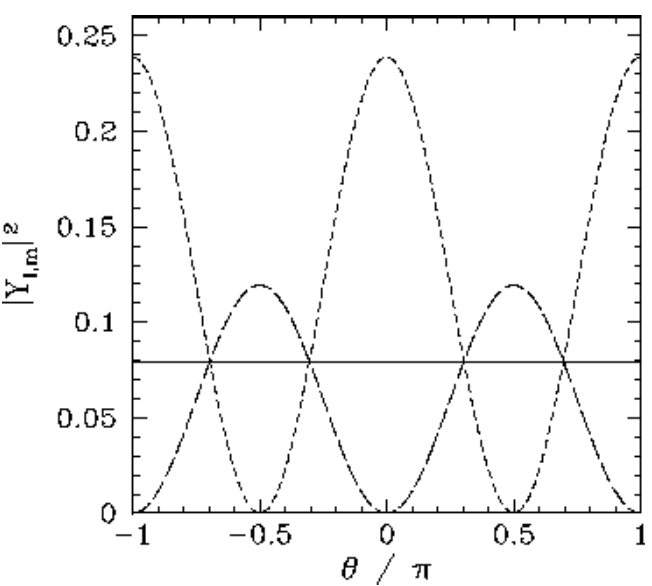
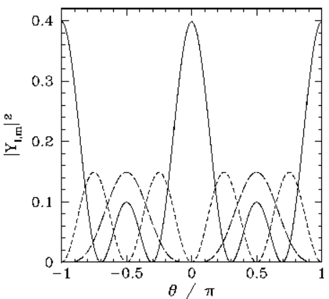
The \(\theta\) variation of these functions is illustrated in Figures [ylm1] and [ylm2].

Figure 18: The \(\left|Y_{l, m}(\theta, \phi)\right|^2\) plotted as a functions of \(\theta\). The solid, short-dashed, and long-dashed curves correspond to \(l, m=0,0, \text { and } 1,0, \text { and } 1,\pm 1\), respectively.

Figure 19: The \(\left|Y_{l, m}(\theta, \phi)\right|^2\) plotted as a functions of \(\theta\). The solid, short-dashed, and long-dashed curves correspond to \(l, m=2,0, \text { and } 2,\pm 1, \text { and } 2,\pm 2\) respectively.