11.9: Zeeman Effect
- Page ID
- 15942
\( \newcommand{\vecs}[1]{\overset { \scriptstyle \rightharpoonup} {\mathbf{#1}} } \)
\( \newcommand{\vecd}[1]{\overset{-\!-\!\rightharpoonup}{\vphantom{a}\smash {#1}}} \)
\( \newcommand{\id}{\mathrm{id}}\) \( \newcommand{\Span}{\mathrm{span}}\)
( \newcommand{\kernel}{\mathrm{null}\,}\) \( \newcommand{\range}{\mathrm{range}\,}\)
\( \newcommand{\RealPart}{\mathrm{Re}}\) \( \newcommand{\ImaginaryPart}{\mathrm{Im}}\)
\( \newcommand{\Argument}{\mathrm{Arg}}\) \( \newcommand{\norm}[1]{\| #1 \|}\)
\( \newcommand{\inner}[2]{\langle #1, #2 \rangle}\)
\( \newcommand{\Span}{\mathrm{span}}\)
\( \newcommand{\id}{\mathrm{id}}\)
\( \newcommand{\Span}{\mathrm{span}}\)
\( \newcommand{\kernel}{\mathrm{null}\,}\)
\( \newcommand{\range}{\mathrm{range}\,}\)
\( \newcommand{\RealPart}{\mathrm{Re}}\)
\( \newcommand{\ImaginaryPart}{\mathrm{Im}}\)
\( \newcommand{\Argument}{\mathrm{Arg}}\)
\( \newcommand{\norm}[1]{\| #1 \|}\)
\( \newcommand{\inner}[2]{\langle #1, #2 \rangle}\)
\( \newcommand{\Span}{\mathrm{span}}\) \( \newcommand{\AA}{\unicode[.8,0]{x212B}}\)
\( \newcommand{\vectorA}[1]{\vec{#1}} % arrow\)
\( \newcommand{\vectorAt}[1]{\vec{\text{#1}}} % arrow\)
\( \newcommand{\vectorB}[1]{\overset { \scriptstyle \rightharpoonup} {\mathbf{#1}} } \)
\( \newcommand{\vectorC}[1]{\textbf{#1}} \)
\( \newcommand{\vectorD}[1]{\overrightarrow{#1}} \)
\( \newcommand{\vectorDt}[1]{\overrightarrow{\text{#1}}} \)
\( \newcommand{\vectE}[1]{\overset{-\!-\!\rightharpoonup}{\vphantom{a}\smash{\mathbf {#1}}}} \)
\( \newcommand{\vecs}[1]{\overset { \scriptstyle \rightharpoonup} {\mathbf{#1}} } \)
\( \newcommand{\vecd}[1]{\overset{-\!-\!\rightharpoonup}{\vphantom{a}\smash {#1}}} \)
\(\newcommand{\avec}{\mathbf a}\) \(\newcommand{\bvec}{\mathbf b}\) \(\newcommand{\cvec}{\mathbf c}\) \(\newcommand{\dvec}{\mathbf d}\) \(\newcommand{\dtil}{\widetilde{\mathbf d}}\) \(\newcommand{\evec}{\mathbf e}\) \(\newcommand{\fvec}{\mathbf f}\) \(\newcommand{\nvec}{\mathbf n}\) \(\newcommand{\pvec}{\mathbf p}\) \(\newcommand{\qvec}{\mathbf q}\) \(\newcommand{\svec}{\mathbf s}\) \(\newcommand{\tvec}{\mathbf t}\) \(\newcommand{\uvec}{\mathbf u}\) \(\newcommand{\vvec}{\mathbf v}\) \(\newcommand{\wvec}{\mathbf w}\) \(\newcommand{\xvec}{\mathbf x}\) \(\newcommand{\yvec}{\mathbf y}\) \(\newcommand{\zvec}{\mathbf z}\) \(\newcommand{\rvec}{\mathbf r}\) \(\newcommand{\mvec}{\mathbf m}\) \(\newcommand{\zerovec}{\mathbf 0}\) \(\newcommand{\onevec}{\mathbf 1}\) \(\newcommand{\real}{\mathbb R}\) \(\newcommand{\twovec}[2]{\left[\begin{array}{r}#1 \\ #2 \end{array}\right]}\) \(\newcommand{\ctwovec}[2]{\left[\begin{array}{c}#1 \\ #2 \end{array}\right]}\) \(\newcommand{\threevec}[3]{\left[\begin{array}{r}#1 \\ #2 \\ #3 \end{array}\right]}\) \(\newcommand{\cthreevec}[3]{\left[\begin{array}{c}#1 \\ #2 \\ #3 \end{array}\right]}\) \(\newcommand{\fourvec}[4]{\left[\begin{array}{r}#1 \\ #2 \\ #3 \\ #4 \end{array}\right]}\) \(\newcommand{\cfourvec}[4]{\left[\begin{array}{c}#1 \\ #2 \\ #3 \\ #4 \end{array}\right]}\) \(\newcommand{\fivevec}[5]{\left[\begin{array}{r}#1 \\ #2 \\ #3 \\ #4 \\ #5 \\ \end{array}\right]}\) \(\newcommand{\cfivevec}[5]{\left[\begin{array}{c}#1 \\ #2 \\ #3 \\ #4 \\ #5 \\ \end{array}\right]}\) \(\newcommand{\mattwo}[4]{\left[\begin{array}{rr}#1 \amp #2 \\ #3 \amp #4 \\ \end{array}\right]}\) \(\newcommand{\laspan}[1]{\text{Span}\{#1\}}\) \(\newcommand{\bcal}{\cal B}\) \(\newcommand{\ccal}{\cal C}\) \(\newcommand{\scal}{\cal S}\) \(\newcommand{\wcal}{\cal W}\) \(\newcommand{\ecal}{\cal E}\) \(\newcommand{\coords}[2]{\left\{#1\right\}_{#2}}\) \(\newcommand{\gray}[1]{\color{gray}{#1}}\) \(\newcommand{\lgray}[1]{\color{lightgray}{#1}}\) \(\newcommand{\rank}{\operatorname{rank}}\) \(\newcommand{\row}{\text{Row}}\) \(\newcommand{\col}{\text{Col}}\) \(\renewcommand{\row}{\text{Row}}\) \(\newcommand{\nul}{\text{Nul}}\) \(\newcommand{\var}{\text{Var}}\) \(\newcommand{\corr}{\text{corr}}\) \(\newcommand{\len}[1]{\left|#1\right|}\) \(\newcommand{\bbar}{\overline{\bvec}}\) \(\newcommand{\bhat}{\widehat{\bvec}}\) \(\newcommand{\bperp}{\bvec^\perp}\) \(\newcommand{\xhat}{\widehat{\xvec}}\) \(\newcommand{\vhat}{\widehat{\vvec}}\) \(\newcommand{\uhat}{\widehat{\uvec}}\) \(\newcommand{\what}{\widehat{\wvec}}\) \(\newcommand{\Sighat}{\widehat{\Sigma}}\) \(\newcommand{\lt}{<}\) \(\newcommand{\gt}{>}\) \(\newcommand{\amp}{&}\) \(\definecolor{fillinmathshade}{gray}{0.9}\)Consider a hydrogen atom placed in a uniform \(z\)-directed external magnetic field of magnitude \(|{\bf B}|\). The modification to the Hamiltonian of the system is \[H_1 = -\mu\cdot{\bf B},\] where \[\mu = - \frac{e}{2\,m_e}\,({\bf L} + 2\,{\bf S})\] is the total electron magnetic moment, including both orbital and spin contributions. [See Equations ([e10.57])–([e10.59]).] Thus, \[H_1 = \frac{e\,B}{2\,m_e}\,(L_z+ 2\,S_z).\]
Suppose that the applied magnetic field is much weaker than the atom’s internal magnetic field, ([e12.124]). Because the magnitude of the internal field is about 25 tesla, this is a fairly reasonable assumption. In this situation, we can treat \(H_1\) as a small perturbation acting on the simultaneous eigenstates of the unperturbed Hamiltonian and the fine structure Hamiltonian. Of course, these states are the simultaneous eigenstates of \(L^2\), \(S^2\), \(J^{\,2}\), and \(J_z\). (See the previous section.) Hence, from standard perturbation theory, the first-order energy-shift induced by a weak external magnetic field is \[\begin{aligned} {\mit\Delta} E_{l,1/2;j,m_j} &= \langle l,1/2;j,m_j|H_1|l,1/2;j,m_j\rangle\nonumber\\[0.5ex] &= \frac{e\,B}{2\,m_e}\,\left(m_j\,\hbar + \langle l,1/2;j,m_j|S_z|l,1/2;j,m_j\rangle\right),\end{aligned}\] because \(J_z=L_z+S_z\). Now, according to Equations ([e11.47]) and ([e11.48]),
\[\label{e12.143} \psi^{(2)}_{j,m_j} = \left(\frac{j+m_j}{2\,l+1}\right)^{1/2}\psi^{(1)}_{m_j-1/2,1/2} + \left(\frac{j-m_j}{2\,l+1}\right)^{1/2}\,\psi^{(1)}_{m_j+1/2,-1/2}\] when \(j=l+1/2\), and \[\psi^{(2)}_{j,m_j} = \left(\frac{j+1-m_j}{2\,l+1}\right)^{1/2}\psi^{(1)}_{m_j-1/2,1/2} - \left(\frac{j+1+m_j}{2\,l+1}\right)^{1/2}\,\psi^{(1)}_{m_j+1/2,-1/2}\] when \(j=l-1/2\). Here, the \(\psi^{(1)}_{m,m_s}\) are the simultaneous eigenstates of \(L^2\), \(S^2\), \(L_z\), and \(S_z\), whereas the \(\psi^{(2)}_{j,m_j}\) are the simultaneous eigenstates of \(L^2\), \(S^2\), \(J^{\,2}\), and \(J_z\). In particular, \[\label{e12.145} S_z\,\psi^{(1)}_{m,\pm 1/2} = \pm \frac{\hbar}{2}\,\psi^{(1)}_{m,\pm 1/2}.\] It follows from Equations ([e12.143])–([e12.145]), and the orthormality of the \(\psi^{(1)}\), that \[\langle l,1/2;j,m_j|S_z|l,1/2;j,m_j\rangle = \pm \frac{m_j\,\hbar}{2\,l+1}\] when \(j=l\pm 1/2\). Thus, the induced energy-shift when a hydrogen atom is placed in an external magnetic field—which is known as the Zeeman effect —becomes \[\label{e12.147} {\mit\Delta} E_{l,1/2;j,m_j} = \mu_B\,B\,m_j\left(1\pm \frac{1}{2\,l+1}\right)\] where the \(\pm\) signs correspond to \(j=l\pm 1/2\). Here, \[\mu_B = \frac{e\,\hbar}{2\,m_e} = 5.788\times 10^{-5}\,{\rm eV/T}\] is known as the Bohr magnetron. Of course, the quantum number \(m_j\) takes values differing by unity in the range \(-j\) to \(j\). It, thus, follows from Equation ([e12.147]) that the Zeeman effect splits degenerate states characterized by \(j=l+1/2\) into \(2\,j+1\) equally spaced states of interstate spacing \[\label{e12.149} {\mit\Delta} E_{j=l+1/2} = \mu_B\,B\left(\frac{2\,l+2}{2\,l+1}\right).\] Likewise, the Zeeman effect splits degenerate states characterized by \(j=l-1/2\) into \(2\,j+1\) equally spaced states of interstate spacing \[\label{e12.150} {\mit\Delta} E_{j=l-1/2} = \mu_B\,B\left(\frac{2\,l}{2\,l+1}\right).\]
In conclusion, in the presence of a weak external magnetic field, the two degenerate \(1S_{1/2}\) states of the hydrogen atom are split by \(2\,\mu_B\,B\). Likewise, the four degenerate \(2S_{1/2}\) and \(2P_{1/2}\) states are split by \((2/3)\,\mu_B\,B\), whereas the four degenerate \(2P_{3/2}\) states are split by \((4/3)\,\mu_B\,B\). This is illustrated in Figure [fzee]. Note, finally, that because the \(\psi^{(2)}_{l,m_j}\) are not simultaneous eigenstates of the unperturbed and perturbing Hamiltonians, Equations ([e12.149]) and ([e12.150]) can only be regarded as the expectation values of the magnetic-field induced energy-shifts. However, as long as the external magnetic field is much weaker than the internal magnetic field, these expectation values are almost identical to the actual measured values of the energy-shifts.
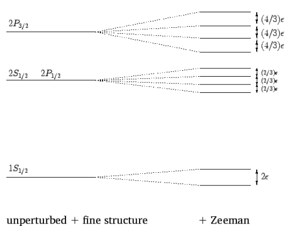
Figure 24: The Zeeman effect for the and states of a hydrogen atom. Here, \(\begin{equation}\epsilon=\mu_{B} B\end{equation}\). Not to scale.
Contributors and Attributions
Richard Fitzpatrick (Professor of Physics, The University of Texas at Austin)
\( \newcommand {\ltapp} {\stackrel {_{\normalsize<}}{_{\normalsize \sim}}}\) \(\newcommand {\gtapp} {\stackrel {_{\normalsize>}}{_{\normalsize \sim}}}\) \(\newcommand {\btau}{\mbox{\boldmath$\tau$}}\) \(\newcommand {\bmu}{\mbox{\boldmath$\mu$}}\) \(\newcommand {\bsigma}{\mbox{\boldmath$\sigma$}}\) \(\newcommand {\bOmega}{\mbox{\boldmath$\Omega$}}\) \(\newcommand {\bomega}{\mbox{\boldmath$\omega$}}\) \(\newcommand {\bepsilon}{\mbox{\boldmath$\epsilon$}}\)