
8.3: Note on the WKB Connection Formula
- Page ID
- 5671

\( \newcommand{\vecs}[1]{\overset { \scriptstyle \rightharpoonup} {\mathbf{#1}} } \)
\( \newcommand{\vecd}[1]{\overset{-\!-\!\rightharpoonup}{\vphantom{a}\smash {#1}}} \)
\( \newcommand{\id}{\mathrm{id}}\) \( \newcommand{\Span}{\mathrm{span}}\)
( \newcommand{\kernel}{\mathrm{null}\,}\) \( \newcommand{\range}{\mathrm{range}\,}\)
\( \newcommand{\RealPart}{\mathrm{Re}}\) \( \newcommand{\ImaginaryPart}{\mathrm{Im}}\)
\( \newcommand{\Argument}{\mathrm{Arg}}\) \( \newcommand{\norm}[1]{\| #1 \|}\)
\( \newcommand{\inner}[2]{\langle #1, #2 \rangle}\)
\( \newcommand{\Span}{\mathrm{span}}\)
\( \newcommand{\id}{\mathrm{id}}\)
\( \newcommand{\Span}{\mathrm{span}}\)
\( \newcommand{\kernel}{\mathrm{null}\,}\)
\( \newcommand{\range}{\mathrm{range}\,}\)
\( \newcommand{\RealPart}{\mathrm{Re}}\)
\( \newcommand{\ImaginaryPart}{\mathrm{Im}}\)
\( \newcommand{\Argument}{\mathrm{Arg}}\)
\( \newcommand{\norm}[1]{\| #1 \|}\)
\( \newcommand{\inner}[2]{\langle #1, #2 \rangle}\)
\( \newcommand{\Span}{\mathrm{span}}\) \( \newcommand{\AA}{\unicode[.8,0]{x212B}}\)
\( \newcommand{\vectorA}[1]{\vec{#1}} % arrow\)
\( \newcommand{\vectorAt}[1]{\vec{\text{#1}}} % arrow\)
\( \newcommand{\vectorB}[1]{\overset { \scriptstyle \rightharpoonup} {\mathbf{#1}} } \)
\( \newcommand{\vectorC}[1]{\textbf{#1}} \)
\( \newcommand{\vectorD}[1]{\overrightarrow{#1}} \)
\( \newcommand{\vectorDt}[1]{\overrightarrow{\text{#1}}} \)
\( \newcommand{\vectE}[1]{\overset{-\!-\!\rightharpoonup}{\vphantom{a}\smash{\mathbf {#1}}}} \)
\( \newcommand{\vecs}[1]{\overset { \scriptstyle \rightharpoonup} {\mathbf{#1}} } \)
\( \newcommand{\vecd}[1]{\overset{-\!-\!\rightharpoonup}{\vphantom{a}\smash {#1}}} \)
\(\newcommand{\avec}{\mathbf a}\) \(\newcommand{\bvec}{\mathbf b}\) \(\newcommand{\cvec}{\mathbf c}\) \(\newcommand{\dvec}{\mathbf d}\) \(\newcommand{\dtil}{\widetilde{\mathbf d}}\) \(\newcommand{\evec}{\mathbf e}\) \(\newcommand{\fvec}{\mathbf f}\) \(\newcommand{\nvec}{\mathbf n}\) \(\newcommand{\pvec}{\mathbf p}\) \(\newcommand{\qvec}{\mathbf q}\) \(\newcommand{\svec}{\mathbf s}\) \(\newcommand{\tvec}{\mathbf t}\) \(\newcommand{\uvec}{\mathbf u}\) \(\newcommand{\vvec}{\mathbf v}\) \(\newcommand{\wvec}{\mathbf w}\) \(\newcommand{\xvec}{\mathbf x}\) \(\newcommand{\yvec}{\mathbf y}\) \(\newcommand{\zvec}{\mathbf z}\) \(\newcommand{\rvec}{\mathbf r}\) \(\newcommand{\mvec}{\mathbf m}\) \(\newcommand{\zerovec}{\mathbf 0}\) \(\newcommand{\onevec}{\mathbf 1}\) \(\newcommand{\real}{\mathbb R}\) \(\newcommand{\twovec}[2]{\left[\begin{array}{r}#1 \\ #2 \end{array}\right]}\) \(\newcommand{\ctwovec}[2]{\left[\begin{array}{c}#1 \\ #2 \end{array}\right]}\) \(\newcommand{\threevec}[3]{\left[\begin{array}{r}#1 \\ #2 \\ #3 \end{array}\right]}\) \(\newcommand{\cthreevec}[3]{\left[\begin{array}{c}#1 \\ #2 \\ #3 \end{array}\right]}\) \(\newcommand{\fourvec}[4]{\left[\begin{array}{r}#1 \\ #2 \\ #3 \\ #4 \end{array}\right]}\) \(\newcommand{\cfourvec}[4]{\left[\begin{array}{c}#1 \\ #2 \\ #3 \\ #4 \end{array}\right]}\) \(\newcommand{\fivevec}[5]{\left[\begin{array}{r}#1 \\ #2 \\ #3 \\ #4 \\ #5 \\ \end{array}\right]}\) \(\newcommand{\cfivevec}[5]{\left[\begin{array}{c}#1 \\ #2 \\ #3 \\ #4 \\ #5 \\ \end{array}\right]}\) \(\newcommand{\mattwo}[4]{\left[\begin{array}{rr}#1 \amp #2 \\ #3 \amp #4 \\ \end{array}\right]}\) \(\newcommand{\laspan}[1]{\text{Span}\{#1\}}\) \(\newcommand{\bcal}{\cal B}\) \(\newcommand{\ccal}{\cal C}\) \(\newcommand{\scal}{\cal S}\) \(\newcommand{\wcal}{\cal W}\) \(\newcommand{\ecal}{\cal E}\) \(\newcommand{\coords}[2]{\left\{#1\right\}_{#2}}\) \(\newcommand{\gray}[1]{\color{gray}{#1}}\) \(\newcommand{\lgray}[1]{\color{lightgray}{#1}}\) \(\newcommand{\rank}{\operatorname{rank}}\) \(\newcommand{\row}{\text{Row}}\) \(\newcommand{\col}{\text{Col}}\) \(\renewcommand{\row}{\text{Row}}\) \(\newcommand{\nul}{\text{Nul}}\) \(\newcommand{\var}{\text{Var}}\) \(\newcommand{\corr}{\text{corr}}\) \(\newcommand{\len}[1]{\left|#1\right|}\) \(\newcommand{\bbar}{\overline{\bvec}}\) \(\newcommand{\bhat}{\widehat{\bvec}}\) \(\newcommand{\bperp}{\bvec^\perp}\) \(\newcommand{\xhat}{\widehat{\xvec}}\) \(\newcommand{\vhat}{\widehat{\vvec}}\) \(\newcommand{\uhat}{\widehat{\uvec}}\) \(\newcommand{\what}{\widehat{\wvec}}\) \(\newcommand{\Sighat}{\widehat{\Sigma}}\) \(\newcommand{\lt}{<}\) \(\newcommand{\gt}{>}\) \(\newcommand{\amp}{&}\) \(\definecolor{fillinmathshade}{gray}{0.9}\)Semiclassical Analysis of a Particle Trapped in a Well in One Dimension
The WKB semiclassical approximate solution to Schrödinger’s equation, \[ \psi(x)=\psi(x_0)\sqrt{\frac{p(x_0)}{p(x)}}\exp\left( \pm \frac{i}{\hbar} \int_{x_0}^x p(x')dx'\right) \tag{8.3.1}\]
is reliable in regions where the wavelength (for oscillating solutions) or the decay length (for exponential solutions) changes only slightly over a distance of one wavelength or decay length respectively. For a particle trapped in a (one-dimensional) potential well, classically the particle would bounce back and forth between the two turning points where its kinetic energy vanishes. In the quantum case, these are precisely the points where the wavelength becomes infinite, so the WKB solution fails.
Taking the Potential Near the Turning Points to be Linear…
However, for a reasonably smooth potential it may be an adequate approximation to treat a turning point region as one where the potential is increasing linearly with distance over a sufficient range that beyond this point the WKB approximation can be used in both directions. The solution of Schrödinger’s equation for a linearly increasing or decreasing potential is well known, it is the Airy function, the solution of the differential equation
\[ \frac{d^2y}{dx^2}+xy=0 \tag{8.3.2}\]
plotted here at the left-hand turning point :
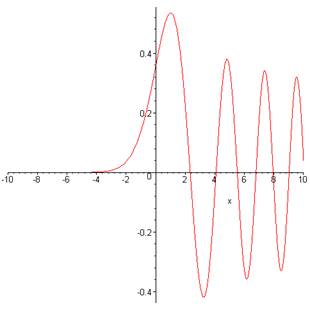
The strategy is to evaluate this function for large \(x\), both positive and negative, so that we can join together the two WKB solutions, valid in the far regions, in a quantitative fashion.
Following Mathews and Walker (page 116) the differential equation is most simply solved by taking its Fourier transform. If
\[ g(\omega)=\int_{-\infty}^{\infty}y(x)e^{-i\omega x}dx, \tag{8.3.3}\]
then \[ -\omega^2g(\omega)+i\frac{dg}{d\omega}=0, \; so \; g(\omega)=Ae^{-i(\omega^3/3)}. \tag{8.3.4}\]
Therefore \[ y(x)=A\int_{-\infty}^{\infty}\frac{d\omega}{2\pi} \exp\left[ i\left( \omega x-\frac{\omega^3}{3}\right) \right]. \tag{8.3.5}\]
Keeping a Low Profile …
This is an exact result, but a nontrivial integral! Fortunately, we are only interested in its value for large values of \(|x|\), and this is precisely where saddlepoint methods become accurate: the contour is distorted to be as low-lying as possible, then the only significant contributions to the integral (thanks to the exponential variation of the amplitude) are from those places where we must go over a saddlepoint to get from one valley to the next. To see where the saddlepoints are, and how they relate to an integral along the real axis, we plot below contour maps of the absolute value of the term in the exponential.
Large positive \(x\): In the map below, we take \(x=10\) (rather small), so the saddlepoints are at \(\pm \sqrt{10}\). If the path of integration is moved down from the real axis into the (dark) valleys (so the integrand becomes exponentially smaller) the contour from \(-\infty\) will come up from the bottom left to the left saddlepoint, over the saddle into the top center valley, then back over the second saddlepoint into the bottom right valley and on to \(+\infty\).
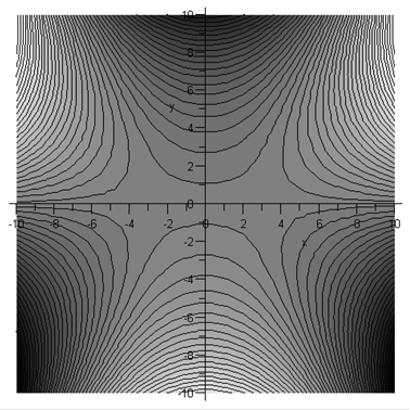
Lighter color means higher ground.
Writing the integral as
\[ \int_{-\infty}^{\infty}e^{f(\omega)}d\omega \tag{8.3.6}\]
(dropping irrelevant overall constants) then
\[ f(\omega)=i\left( \omega x-\frac{\omega^3}{3}\right),\; f'(\omega)=i(x-\omega^2) \; and\; f"(\omega)=-2i\omega. \tag{8.3.7}\]
(Mathews and Walker take the “large” parameter \(x\) out of \(f\), we’ve left it in—this doesn’t affect the final result.) Near the positive saddlepoint
\[ f(\omega)=f(\sqrt{x})+\frac{1}{2}f''(\sqrt{x})(\omega-\sqrt{x})^2=i\frac{2}{3}x^{3/2}-i\sqrt{x}(\omega-\sqrt{x})^2 \tag{8.3.8}\]
dropping higher-order terms. Since \(f′′\) is pure imaginary at the saddlepoint, the appropriate path for a real exponent in the Gaussian integral is at \(\pi /4\) to the x- axis. So in the path integral
\[ dz=e^{\pm i\pi /4} ds \tag{8.3.9}\]
where \(ds\) is a real parameter measuring incremental path length, and the sign in the exponent is positive for the saddlepoint on the left. The contributions from the two saddlepoints give the asymptotic (large positive \(x\) ) solutions as:
\[ y(x)\sim \frac{2\sqrt{\pi}}{x^{1/4}}\cos\left( \frac{2}{3}x^{3/2}-\frac{\pi}{4}\right). \tag{8.3.10}\]
Large negative \(x\): In this case, the saddlepoint geography is quite different, although the distant geography is the same, being dominated by the \(\omega^3\) term.
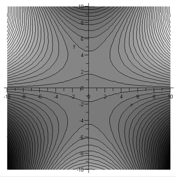
Just as before, the real axis integration path can be moved down from the real axis into the valleys at bottom left and bottom right. (The extra contributions from linking up the new path with the real axis at infinity are zero.) It is clear from the map above that to get from the valley on the left to the one on the right means just going over the saddlepoint on the negative imaginary axis. Note from the darker shading that the other saddlepoint is at higher elevation.
The integration through the saddlepoint is parallel to the real axis, and gives \[ y(x)\sim \frac{\sqrt{\pi}}{(-x)^{1/4}}\exp\left[ -\frac{2}{3}(-x)^{3/2}\right]. \tag{8.3.11}\]
This, then, is the decaying wavefunction solution of the Airy equation that we are looking for, and it is clear that it goes smoothly from this exponential to the cosine form \[ y(x)\sim \frac{2\sqrt{\pi}}{x^{1/4}}\cos\left( \frac{2}{3}x^{3/2}-\frac{\pi}{4}\right). \tag{8.3.10}\]
as \(x\) is taken along the real axis from large negative to large positive values.
Landau's Quick Method
Incidentally, Landau gives a quick way to see how these formulas connect. These are asymptotic solutions to the original Airy equation, valid as long as \(x\) is well away from the origin. But we can go from one to the other, avoiding the origin, if we regard \(x\) as a complex variable and move out into the complex plane—Landau takes a semicircle in the upper half plane, begins with the exponentially decaying solution now written
\[ y(\rho e^{i\phi})\sim \frac{\sqrt{\pi}}{(-\rho e^{i\phi})^{1/4}}\exp\left[ -\frac{2}{3}\rho^{3/2}\left( \cos\frac{3}{2}\phi+i\sin\frac{3}{2}\phi \right) \right] \tag{8.3.12}\]
the phase \(\phi\) varying from 0 to \(\pi\). The exponential factor at first increases in modulus, then becomes pure imaginary, exactly equal to one of the two terms in the cosine form for positive \(x\).
If one takes the cosine formula and continues it into the upper half complex plane, one term grows exponentially, the other goes to zero. Suppose one begins at some large value of \(x\) and moves in a circle around \(x=0\) back to the now negative real axis. This will give \[ y(x)\sim \frac{\sqrt{\pi}}{(x)^{1/4}}\exp i\left( \frac{2}{3}(x)^{3/2}-\sqrt{\pi}{4}\right). \tag{8.3.13}\]
This is actually the same as the expression we already derived: the \(\pi /4\) cancels against the minus sign inside the fourth root, the \(i\) against the minus sign raised to the \(3/2\) power.