
1.5: The Scattering Amplitude and Scattering Cross Section
- Page ID
- 34592

We can use the results of the previous section to systematically characterize the outcomes of a scattering experiment. Let the incident wavefunction be a plane wave,
\[\psi_i(\mathbf{r}) = \Psi_i \, e^{i\mathbf{k}_i\cdot\mathbf{r}},\]
in \(d\)-dimensional space. Here, \(\Psi_i \in \mathbb{C}\) is the incident wave amplitude, and \(\mathbf{k}_i\) is the incident momentum. Let \(k = |\mathbf{k}_i|\) denote its magnitude, so that the particle energy is \(E = \hbar^2k^2/2m\). We adopt coordinates \((r,\Omega)\), where \(r\) is the distance from the origin. For 1D, \(\Omega \in \pm\) which specifies the choice of “forward” or “backward” scattering; for 2D polar coordinates, \(\Omega = \phi\); and for 3D spherical coordinates, \(\Omega = (\theta,\phi)\).
Far from the origin, the scattered wavefunction reduces to the form
\[\psi_s(\mathbf{r})\; \overset{r\rightarrow\infty}{\longrightarrow}\; \Psi_i \, r^{\frac{1-d}{2}} \, e^{ikr} \, f(\Omega).\]
The complex function \(f(\Omega)\), called the scattering amplitude, is the fundamental quantity of interest in scattering experiments. It describes how the particle is scattered in various directions, depending on the inputs to the problem (i.e., \(\mathbf{k}_i\) and the scattering potential).
Sometimes, we write the scattering amplitude using the alternative notation
\[f(\mathbf{k}_i \rightarrow \mathbf{k}_f), \;\;\;\mathrm{where}\;\; \mathbf{k}_f = k \hat{\mathbf{r}}.\]
This emphasizes firstly that the incident wave-vector is \(\mathbf{k}_i\); and secondly that the particle is scattered in some direction which can be specified by either the unit position vector \(\hat{\mathbf{r}}\), or equivalently by the momentum vector \(\mathbf{k}_f = k \hat{\mathbf{r}}\), or by the angular coordinates \(\Omega\).
From the scattering amplitude, we define two other important quantities of interest:
Definition: Scattering Cross Sections
\[\begin{align} \frac{d\sigma}{d\Omega} &= \big|f(\Omega)\big|^2 \qquad\quad\quad \text{(the } \textbf{differential scattering cross section}) \\ \sigma &= \int d\Omega\; \big|f(\Omega)\big|^2 \quad\; \text{(the }\textbf{total scattering cross section}). \end{align}\]
In the second equation, \(\int d\Omega\) denotes the integral(s) over all the angle coordinates; for 1D, this is instead a discrete sum over the two possible directions, forward and backward.
The term “cross section” comes from an analogy with the scattering of classical particles. Consider the probablity current density associated with the scattered wavefunction:
\[\mathbf{J}_s = \frac{\hbar}{m} \mathrm{Im}\big[\psi_s^*\nabla\psi_s\big].\]
Let us focus only on the \(r\)-component of the current density, in the \(r\rightarrow\infty\) limit:
\[\begin{align}\begin{aligned}J_{s,r}\; &\;\;=\;\;\;\, \frac{\hbar}{m}\, \mathrm{Im}\left[\psi_s^* \frac{\partial}{\partial r}\psi_s\right] \\ &\overset{r\rightarrow\infty}{\longrightarrow}\;\, \frac{\hbar}{m}\; |\Psi_i|^2 \; |f(\Omega)|^2 \mathrm{Im}\left[\left(r^{\frac{1-d}{2}} \, e^{ikr}\right)^* \frac{\partial}{\partial r} \left(r^{\frac{1-d}{2}} \, e^{ikr}\right)\right] \\ & \;\;=\;\;\;\, \frac{\hbar \,k}{m}\; |\Psi_i|^2 \; |f(\Omega)|^2 \,r^{1-d}.\end{aligned}\end{align}\]
The total flux of outgoing probability is obtained by integrating \(J_{s,r}\) over a constant-\(r\) surface:
\[I_s \;=\; \int d\Omega\; r^{d-1} \, J_{s,r} \;=\; \frac{\hbar k}{m} \;|\Psi_i|^2 \; \int d\Omega\; \big|f(\Omega)\big|^2. \label{scatterI}\]
We can assign a physical interpretation to each term in this result. The first factor, \(\hbar k/m\), is the particle’s speed (i.e., the group velocity of the de Broglie wave). The second factor, \(|\Psi_i|^2\), is the probability density of the incident wave, which has units of \([x^{-d}]\) (i.e., inverse \(d\)-dimensional “volume”). The product of these two factors represents the incident flux,
\[J_{i} = \frac{\hbar k}{m} \;|\Psi_i|^2.\]
This has units of \([x^{1-d}t^{-1}]\) (i.e., rate per unit “area”).
Let us re-imagine this incident flux \(J_i\) as a stream of classical particles, and the scatterer as a “hard-body” scatterer that only interacts with those particles striking it directly:
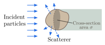
In this classical picture, the rate at which the incident particles strike the scatterer is
\[I_s = J_i \, \sigma,\]
where \(\sigma\) is the exposed cross-sectional area of the scatterer. Comparing this expression to Equation \(\eqref{scatterI}\), we see that \(\int d\Omega\,|f|^2\) plays a role analogous to the classical hard-body cross-sectional area. We hence call
\[\sigma \equiv \int d\Omega\,|f|^2\]
the total scattering cross section. Moreover, the integrand \(|f|^2\) is called the differential scattering cross section, for it represents the rate, per unit of solid angle, at which particles are scattered in a given direction. The total and differential scattering cross sections are the principal observable quantities that can be obtained from scattering experiments.