3.4: Bell's Theorem

In 1964, John S. Bell published a bombshell paper showing that the predictions of quantum theory are inherently inconsistent with hidden variable theories. The amazing thing about this result, known as Bell’s theorem, is that it requires no knowledge about the details of the hidden variable theory, just that it is deterministic and local. Here, we present a simplified version of Bell’s theorem due to Mermin (1981).

We again consider spin-1/2 particle pairs, with particle \(A\) sent to Alice at Alpha Centauri, and particle \(B\) to Bob at Betelgeuse. Each experimentalist can measure the particle’s spin along three distinct choices of spin axis. These spin observables are denoted by \(S_1\), \(S_2\), and \(S_3\). We will not specify the actual directions of these spin axes until later in the proof. For now, just note that the axes need not correspond to orthogonal spatial directions.

We repeatedly prepare the particle pairs in the singlet state

\[|\psi\rangle = \frac{1}{\sqrt{2}} \Big(|\!+\!z\rangle|\!-\!z\rangle \,-\, |\!-\!z\rangle|\!+\!z\rangle\Big),\]

and send the respective particles to Alice and Bob. During each round of the experiment, each experimentalist randomly chooses one of the three spin axes \(S_1\), \(S_2\), or \(S_3\), and performs that spin measurement. It doesn’t matter which experimentalist performs the measurement first; the experimentalists can’t influence each other, as there is not enough time for a light-speed signal to travel between the two locations. Many rounds of the experiment are conducted; for each round, both experimentalists’ choices of spin axis are recorded, along with their measurement results.

Figure \(\PageIndex{1}\)

At the end, the experimental records are brought together and examined. We assume that the results are consistent with the predictions of quantum theory. Among other things, this means that whenever the experimentalists happen to choose the same measurement axis, they always find opposite spins. (For example, this is the case during “Experiment 4” in the above figure, where both experimentalists happened to measure \(S_3\).)

Can a hidden variable theory reproduce the results predicted by quantum theory? In a hidden variable theory, each particle must have a definite value for each spin observable. For example, particle \(A\) might have \(S_1 = +\hbar/2, \, S_2 = +\hbar/2, \, S_3 = -\hbar/2\). Let us denote this by \([++-]\). To be consistent with the predictions of quantum theory, the hidden spin variables for the two particles must have opposite values along each direction. This means that there are \(8\) distinct possibilities, which we can denote as

\[\begin{aligned} \begin{aligned}{[}{+++};{---}], \;\;\; [{++-};{--+}], \;\;\; [{+-+};{-+-}], \;\;\; [{+--};{-++}],\\ [{-++};{+--}], \;\;\; [{-+-};{+-+}], \;\;\; [{--+};{++-}], \;\;\; [{---};{+++}].\end{aligned}\end{aligned}\]

For instance, \([{++-};{--+}]\) indicates that for particle \(A\), \(S_1 = S_2 = +\hbar/2\) and \(S_3 = -\hbar/2\), while particle \(B\) has the opposite spin values, \(S_1 = S_2 = -\hbar/2\) and \(S_3 = +\hbar/2\). So far, however, we don’t know anything about the relative probabilities of these 8 cases.

Let’s now focus on the subset of experiments in which the two experimentalists happened to choose different spin axes (e.g., Alice chose \(S_1\) and Bob chose \(S_2\)). Within this subset, what is the probability for the two measurement results to have opposite signs (i.e., one \(+\) and one \(-\))? To answer this question, we first look at the following 6 cases:

\[\begin{aligned} \begin{aligned}{[}{++-};{--+}], \;\;\; [{+-+};{-+-}], \;\;\; [{+--};{-++}],\\ [{-++};{+--}], \;\;\; [{-+-};{+-+}], \;\;\; [{--+};{++-}].\end{aligned}\end{aligned}\]

These are the cases which do not have all \(+\) or all \(-\) for each particle. Consider one of these, say \({[}{++-};{--+}]\). The two experimentalists picked their measurement axes at random each time, and amongst the experiments where they picked different axes, there are two ways for the measurement results to have opposite signs: \((S_1,S_2)\) or \((S_2,S_1)\). There are four ways to get the same sign: \((S_1,S_3)\), \((S_2,S_3)\), \((S_3,S_1)\) and \((S_3, S_2)\). Thus, for this particular set of hidden variables, the probability for measurement results with opposite signs is 1/3. If we go through all 6 of the cases listed above, we find that in call cases, the probability for opposite signs is 1/3.

Now look at the remaining 2 cases:

\[{[}{+++};{---}], \;\;\; [{---};{+++}].\]

For these, Alice and Bob always obtain results with opposite signs. Combining this with the findings from the previous paragraph, we obtain the following statement:

Given that the two experimentalists choose different spin axes, the probability that their results have opposite signs is \(P \ge 1/3\).

This is called Bell’s inequality. If we can arrange a situation where quantum theory predicts a probability \(P < 1/3\) (i.e., a violation of Bell’s inequality), that would mean that quantum theory is inherently inconsistent with local deterministic hidden variables. This conclusion would hold regardless of the “inner workings” of the hidden variable theory. In particular, note that the above derivation made no assumptions about the relative probabilities of the hidden variable states.

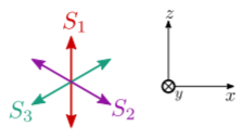
To complete the proof, we must find a set \(\{S_1, S_2, S_3\}\) such that the predictions of quantum mechanics violate Bell’s inequality. One simple choice is to align \(S_1\) with the \(z\) axis, and align \(S_2\) and \(S_3\) along the \(x\)-\(z\) plane at \(120^\circ\) (\(2\pi/3\) radians) from \(S_1\), as shown below:

Figure \(\PageIndex{2}\)

The corresponding spin operators can be written in the eigenbasis of \(\hat{S}_z\):

\[\begin{align} \begin{aligned}\hat{S}_1 &= \frac{\hbar}{2} \, \sigma_3 \\ \hat{S}_2 &= \frac{\hbar}{2} \, \left[\cos(2\pi/3) \sigma_3 + \sin(2\pi/3)\sigma_1\right] \\ \hat{S}_3 &= \frac{\hbar}{2} \, \left[\cos(2\pi/3) \sigma_3 - \sin(2\pi/3)\sigma_1\right].\end{aligned}\end{align}\]

Suppose Alice chooses \(S_1\), and obtains \(+\hbar/2\). Particle \(A\) collapses to state \(|\!+\!z\rangle\), and particle \(B\) collapses to state \(|\!-\!z\rangle\). Bob is assumed to choose a different spin axis. If the choice is \(S_2\), the expectation value is

\[\begin{align} \begin{aligned}\langle\, - z \, | \, S_2 \,|-\!z\,\rangle &= \frac{\hbar}{2} \Big[\cos(2\pi/3) \langle\,- z\,|\sigma_3| - \!z\,\rangle + \sin(2\pi/3)\langle\,- z\,|\sigma_1|-\!z\,\rangle\Big]\\ &= \frac{\hbar}{2} \cdot \frac{1}{2} \end{aligned}\end{align}\]

If \(P_+\) and \(P_-\) respectively denote the probability of measuring \(+\hbar/2\) and \(-\hbar/2\) in this measurement, the above equation implies that \(P_+ - P_- = + 1/2\). Moreover, \(P_+ + P_- = 1\) by probability conservation. Hence, the probability of obtaining a negative value (the opposite sign from Alice’s measurement) is \(P_- = 1/4\). All the other possible scenarios are worked out similarly. The result is that the overall probability of the two experimentalists obtaining opposite results (in the cases where they choose different measurement axis) is \(1/4\). Bell’s inequality is violated!

Last of all, we must consult Nature itself. Is it possible to observe, in an actual experiment, probabilities that violate Bell’s inequality? In the decades following Bell’s 1964 paper, many experiments were performed to answer this question. These experiments are all substantially more complicated than the simple two-particle spin-\(1/2\) model that we’ve studied, and they are subject to various uncertainties and “loopholes” that are beyond the scope of our discussion. But in the end, the experimental consensus appears to be a clear yes: Nature really does behave according to quantum mechanics, and in a manner that cannot be replicated by deterministic local hidden variables! A summary of the experimental evidence is given in a review paper by Aspect (1999).