
9.3: Gravitational Radiation (Part 2)
- Page ID
- 11622

\( \newcommand{\vecs}[1]{\overset { \scriptstyle \rightharpoonup} {\mathbf{#1}} } \)
\( \newcommand{\vecd}[1]{\overset{-\!-\!\rightharpoonup}{\vphantom{a}\smash {#1}}} \)
\( \newcommand{\dsum}{\displaystyle\sum\limits} \)
\( \newcommand{\dint}{\displaystyle\int\limits} \)
\( \newcommand{\dlim}{\displaystyle\lim\limits} \)
\( \newcommand{\id}{\mathrm{id}}\) \( \newcommand{\Span}{\mathrm{span}}\)
( \newcommand{\kernel}{\mathrm{null}\,}\) \( \newcommand{\range}{\mathrm{range}\,}\)
\( \newcommand{\RealPart}{\mathrm{Re}}\) \( \newcommand{\ImaginaryPart}{\mathrm{Im}}\)
\( \newcommand{\Argument}{\mathrm{Arg}}\) \( \newcommand{\norm}[1]{\| #1 \|}\)
\( \newcommand{\inner}[2]{\langle #1, #2 \rangle}\)
\( \newcommand{\Span}{\mathrm{span}}\)
\( \newcommand{\id}{\mathrm{id}}\)
\( \newcommand{\Span}{\mathrm{span}}\)
\( \newcommand{\kernel}{\mathrm{null}\,}\)
\( \newcommand{\range}{\mathrm{range}\,}\)
\( \newcommand{\RealPart}{\mathrm{Re}}\)
\( \newcommand{\ImaginaryPart}{\mathrm{Im}}\)
\( \newcommand{\Argument}{\mathrm{Arg}}\)
\( \newcommand{\norm}[1]{\| #1 \|}\)
\( \newcommand{\inner}[2]{\langle #1, #2 \rangle}\)
\( \newcommand{\Span}{\mathrm{span}}\) \( \newcommand{\AA}{\unicode[.8,0]{x212B}}\)
\( \newcommand{\vectorA}[1]{\vec{#1}} % arrow\)
\( \newcommand{\vectorAt}[1]{\vec{\text{#1}}} % arrow\)
\( \newcommand{\vectorB}[1]{\overset { \scriptstyle \rightharpoonup} {\mathbf{#1}} } \)
\( \newcommand{\vectorC}[1]{\textbf{#1}} \)
\( \newcommand{\vectorD}[1]{\overrightarrow{#1}} \)
\( \newcommand{\vectorDt}[1]{\overrightarrow{\text{#1}}} \)
\( \newcommand{\vectE}[1]{\overset{-\!-\!\rightharpoonup}{\vphantom{a}\smash{\mathbf {#1}}}} \)
\( \newcommand{\vecs}[1]{\overset { \scriptstyle \rightharpoonup} {\mathbf{#1}} } \)
\(\newcommand{\longvect}{\overrightarrow}\)
\( \newcommand{\vecd}[1]{\overset{-\!-\!\rightharpoonup}{\vphantom{a}\smash {#1}}} \)
\(\newcommand{\avec}{\mathbf a}\) \(\newcommand{\bvec}{\mathbf b}\) \(\newcommand{\cvec}{\mathbf c}\) \(\newcommand{\dvec}{\mathbf d}\) \(\newcommand{\dtil}{\widetilde{\mathbf d}}\) \(\newcommand{\evec}{\mathbf e}\) \(\newcommand{\fvec}{\mathbf f}\) \(\newcommand{\nvec}{\mathbf n}\) \(\newcommand{\pvec}{\mathbf p}\) \(\newcommand{\qvec}{\mathbf q}\) \(\newcommand{\svec}{\mathbf s}\) \(\newcommand{\tvec}{\mathbf t}\) \(\newcommand{\uvec}{\mathbf u}\) \(\newcommand{\vvec}{\mathbf v}\) \(\newcommand{\wvec}{\mathbf w}\) \(\newcommand{\xvec}{\mathbf x}\) \(\newcommand{\yvec}{\mathbf y}\) \(\newcommand{\zvec}{\mathbf z}\) \(\newcommand{\rvec}{\mathbf r}\) \(\newcommand{\mvec}{\mathbf m}\) \(\newcommand{\zerovec}{\mathbf 0}\) \(\newcommand{\onevec}{\mathbf 1}\) \(\newcommand{\real}{\mathbb R}\) \(\newcommand{\twovec}[2]{\left[\begin{array}{r}#1 \\ #2 \end{array}\right]}\) \(\newcommand{\ctwovec}[2]{\left[\begin{array}{c}#1 \\ #2 \end{array}\right]}\) \(\newcommand{\threevec}[3]{\left[\begin{array}{r}#1 \\ #2 \\ #3 \end{array}\right]}\) \(\newcommand{\cthreevec}[3]{\left[\begin{array}{c}#1 \\ #2 \\ #3 \end{array}\right]}\) \(\newcommand{\fourvec}[4]{\left[\begin{array}{r}#1 \\ #2 \\ #3 \\ #4 \end{array}\right]}\) \(\newcommand{\cfourvec}[4]{\left[\begin{array}{c}#1 \\ #2 \\ #3 \\ #4 \end{array}\right]}\) \(\newcommand{\fivevec}[5]{\left[\begin{array}{r}#1 \\ #2 \\ #3 \\ #4 \\ #5 \\ \end{array}\right]}\) \(\newcommand{\cfivevec}[5]{\left[\begin{array}{c}#1 \\ #2 \\ #3 \\ #4 \\ #5 \\ \end{array}\right]}\) \(\newcommand{\mattwo}[4]{\left[\begin{array}{rr}#1 \amp #2 \\ #3 \amp #4 \\ \end{array}\right]}\) \(\newcommand{\laspan}[1]{\text{Span}\{#1\}}\) \(\newcommand{\bcal}{\cal B}\) \(\newcommand{\ccal}{\cal C}\) \(\newcommand{\scal}{\cal S}\) \(\newcommand{\wcal}{\cal W}\) \(\newcommand{\ecal}{\cal E}\) \(\newcommand{\coords}[2]{\left\{#1\right\}_{#2}}\) \(\newcommand{\gray}[1]{\color{gray}{#1}}\) \(\newcommand{\lgray}[1]{\color{lightgray}{#1}}\) \(\newcommand{\rank}{\operatorname{rank}}\) \(\newcommand{\row}{\text{Row}}\) \(\newcommand{\col}{\text{Col}}\) \(\renewcommand{\row}{\text{Row}}\) \(\newcommand{\nul}{\text{Nul}}\) \(\newcommand{\var}{\text{Var}}\) \(\newcommand{\corr}{\text{corr}}\) \(\newcommand{\len}[1]{\left|#1\right|}\) \(\newcommand{\bbar}{\overline{\bvec}}\) \(\newcommand{\bhat}{\widehat{\bvec}}\) \(\newcommand{\bperp}{\bvec^\perp}\) \(\newcommand{\xhat}{\widehat{\xvec}}\) \(\newcommand{\vhat}{\widehat{\vvec}}\) \(\newcommand{\uhat}{\widehat{\uvec}}\) \(\newcommand{\what}{\widehat{\wvec}}\) \(\newcommand{\Sighat}{\widehat{\Sigma}}\) \(\newcommand{\lt}{<}\) \(\newcommand{\gt}{>}\) \(\newcommand{\amp}{&}\) \(\definecolor{fillinmathshade}{gray}{0.9}\)In this section we study several examples of exact solutions to the field equations. Each of these can readily be shown not to be a mere coordinate wave, since in each case the Riemann tensor has nonzero elements.
Example 1: An exact solution
We’ve already seen, e.g., in the derivation of the Schwarzschild metric in section 6.2, that once we have an approximate solution to the equations of general relativity, we may be able to find a series solution. Historically this approach was only used as a last resort, because the lack of computers made the calculations too complex to handle, and the tendency was to look for tricks that would make a closed-form solution possible. But today the series method has the advantage that any mere mortal can have some reasonable hope of success with it — and there is nothing more boring (or demoralizing) than laboriously learning someone else’s special trick that only works for a specific problem. In this example, we’ll see that such an approach comes tantalizingly close to providing an exact, oscillatory plane wave solution to the field equations.
Our best solution so far was of the form
\[ds^{2} = dt^{2} - (1 + f) dx^{2} - \frac{dy^{2}}{1 + f} - dz^{2}, \tag{9.2.6}\]
where f = Asin(z − t). This doesn’t seem likely to be an exact solution for large amplitudes, since the x and y coordinates are treated asymmetrically. In the extreme case of |A| ≥ 1, there would be singularities in gyy, but not in gxx. Clearly the metric will have to have some kind of nonlinear dependence on f, but we just haven’t found quite the right nonlinear dependence. Suppose we try something of this form:
\[ds^{2} = dt^{2} - (1 + f + cf^{2}) dx^{2} - (1 - f + df^{2}) dy^{2} - dz^{2} \tag{9.2.7}\]
This approximately conserves volume, since (1+f +. . .)(1−f +. . .) equals unity, up to terms of order f2. The following program tests this form.
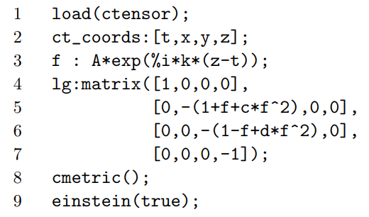
In line 3, the motivation for using the complex exponential rather than a sine wave in f is the usual one of obtaining simpler expressions; as we’ll see, this ends up causing problems. In lines 5 and 6, the symbols c and d have not been defined, and have not been declared as depending on other variables, so Maxima treats them as unknown constants. The result is Gtt ∼ (4d + 4c − 3)A2 for small A, so we can make the A2 term disappear by an appropriate choice of d and c. For symmetry, we choose c = d = \(\frac{3}{8}\). With these values of the constants, the result for Gtt is of order A4. This technique can be extended to higher and higher orders of approximation, resulting in an exact series solution to the field equations.
Unfortunately, the whole story ends up being too good to be true. The resulting metric has complex-valued elements. If general relativity were a linear field theory, then we could apply the usual technique of forming linear combinations of expressions of the form e+i... and e−i..., so as to give a real result. But the field equations of general relativity are nonlinear, so the resulting linear combination is no longer a solution. The best we can do is to make a non-oscillatory real exponential solution (problem 2).
Example 2: An exact, oscillatory, non-monochromatic solution
Assume a metric of the form
\[ds^{2} = dt^{2} - p(z - t)^{2} dx^{2} - q(z - t)^{2} dy^{2} - dz^{2}, \ldots \tag{9.2.8}\]
where p and q are arbitrary functions. Such a metric would clearly represent some kind of transverse-polarized plane wave traveling at velocity c(= 1) in the z direction. The following Maxima code calculates its Einstein tensor.
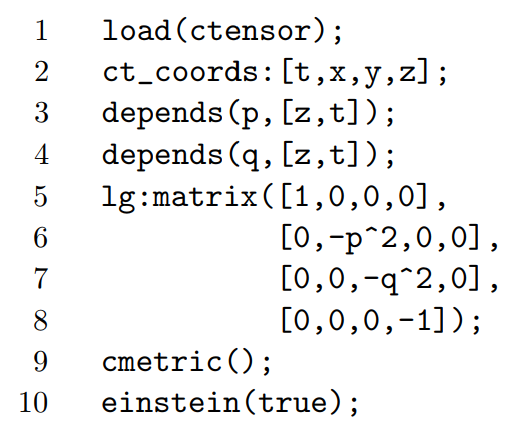
The result is proportional to \(\frac{\ddot{q}}{q} + \frac{\ddot{p}}{p}\), so any functions p and q that satisfy the differential equation \(\frac{\ddot{q}}{q} + \frac{\ddot{p}}{p}\) = 0 will result in a solution to the field equations. Setting p(u) = 1 + Acos u, for example, we find that q is oscillatory, but with a period longer than 2\(\pi\) (problem 3).
Example 3: An exact, plane, monochromatic wave
Any metric of the form
\[ds^{2} = (1 - h) dt^{2} - dx^{2} - dy^{2} - (1 + h) dz^{2} + 2hdzdt, \tag{9.2.9}\]
where h = f(z − t)xy, and f is any function, is an exact solution of the field equations (problem 4).
Because h is proportional to xy, this does not appear at first glance to be a uniform plane wave. One can verify, however, that all the components of the Riemann tensor depend only on z − t, not on x or y. Therefore there is no measurable property of this metric that varies with x and y.
Rate of Radiation
How can we find the rate of gravitational radiation from a system such as the Hulse-Taylor pulsar?
Let’s proceed by analogy. The simplest source of sound waves is something like the cone of a stereo speaker. Since typical sound waves have wavelengths measured in meters, the entire speaker is generally small compared to the wavelength. The speaker cone is a surface of oscillating displacement \(x = x_o \sin \omega t\). Idealizing such a source to a radially pulsating spherical surface, we have an oscillating monopole that radiates sound waves uniformly in all directions. To find the power radiated, we note that the velocity of the source-surface is proportional to xo\(\omega\), so the kinetic energy of the air immediately in contact with it is proportional to \(\omega^{2}x^2_o\). The power radiated is therefore proportional to \(\omega^{2} x^2_o\).
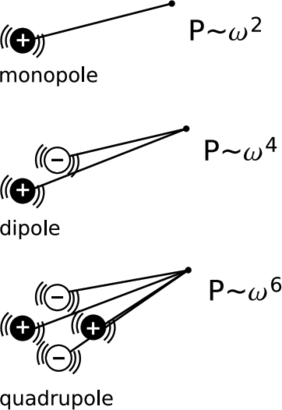
In electromagnetism, conservation of charge forbids the existence of an oscillating electric monopole. The simplest radiating source is therefore an oscillating electric dipole D = Do sin \(\omega\)t. If the dipole’s physical size is small compared to a wavelength of the radiation, then the radiation is an inefficient process; at any point in space, there is only a small difference in path length between the positive and negative portions of the dipole, so there tends to be strong cancellation of their contributions, which were emitted with opposite phases. The result is that the wave’s electromagnetic potential four-vector (Section 4.2) is proportional to Do\(\omega\), the fields to Do\(\omega^{2}\), and the radiated power to D2o\(\omega^{4}\). The factor of \(\omega^{4}\) can be broken down into (\(\omega^{2}\))(\(\omega^{2}\)), where the first factor of \(\omega^{2}\) occurs for reasons similar to the ones that explain the \(\omega^{2}\) factor for the monopole radiation of sound, while the second \(\omega^{2}\) arises because the smaller ω is, the longer the wavelength, and the greater the inefficiency in radiation caused by the small size of the source compared to the wavelength.
Example 4: am radio
Commercial AM radio uses wavelengths of several hundred meters, so AM dipole antennas are usually orders of magnitude shorter than a wavelength. This causes severe attenuation in both transmission and reception. (There are theorems called reciprocity theorems that relate efficiency of transmission to efficiency of reception.) Receivers therefore need to use of a large amount of amplification. This doesn’t cause problems, because the ambient sources of RF noise are attenuated by the short antenna just as severely as the signal.
Since our universe doesn’t seem to have particles with negative mass, we can’t form a gravitational dipole by putting positive and negative masses on opposite ends of a stick — and furthermore, such a stick will not spin freely about its center, because its center of mass does not lie at its center! In a more realistic system, such as the Hulse-Taylor pulsar, we have two unequal masses orbiting about their common center of mass. By conservation of momentum, the mass dipole moment of such a system is constant, so we cannot have an oscillating mass dipole. The simplest source of gravitational radiation is therefore an oscillating mass quadrupole, Q = Qo sin \(\omega\)t. As in the case of the oscillating electric dipole, the radiation is suppressed if, as is usually the case, the source is small compared to the wavelength. The suppression is even stronger in the case of a quadrupole, and the result is that the radiated power is proportional to Q2o\(\omega^{6}\).
This result has the interesting property of being invariant under a rescaling of coordinates. In geometrized units, mass, distance, and time all have the same units, so that Q2o has units of (length3)2 while \(\omega^{6}\) has units of (length)−6. This is exactly what is required, because in geometrized units, power is unitless, energy/time = length/length = 1.
We can also tie the \(\omega^{6}\) dependence to our earlier argument for the dissipation of energy by gravitational waves. The argument was that gravitating bodies are subject to time-delayed gravitational forces, with the result that orbits tend to decay. This argument only works if the forces are time-varying; if the forces are constant over time, then the time delay has no effect. For example, in the semi-Newtonian limit the field of a sheet of mass is independent of distance from the sheet. (The electrical analog of this fact is easily proved using Gauss’s law.) If two parallel sheets fall toward one another, then neither is subject to a time-varying force, so there will be no radiation. In general, we expect that there will be no gravitational radiation from a particle unless the third derivative of its position d3 x/ dt 3 is nonzero. (The same is true for electric quadrupole radiation.) In the special case where the position oscillates sinusoidally, the chain rule tells us that taking the third derivative is equivalent to bringing out a factor of \(\omega^{3}\). Since the amplitude of gravitational waves is proportional to \(\frac{d^{3} x}{dt^{3}}\), their energy varies as (\(\frac{d^{3} x}{dt^{3}}\))2, or \(\omega^{6}\).
The general pattern we have observed is that for multipole radiation of order m (0=monopole, 1=dipole, 2=quadrupole), the radiated power depends on \(\omega^{2(m+1)}\). Since gravitational radiation must always have m = 2 or higher, we have the very steep \(\omega^{6}\) dependence of power on frequency. This demonstrates that if we want to see strong gravitational radiation, we need to look at systems that are oscillating extremely rapidly. For a binary system with unequal masses of order m, with orbits having radii of order r, we have Qo ∼ mr2 . Newton’s laws give \(\omega\) ∼ m1/2r−3/2, which is essentially Kepler’s law of periods. The result is that the radiated power should depend on (\(\frac{m}{r}\))5. Reinserting the proper constants to give an equation that allows practical calculation in SI units, we have
\[P = k \frac{G^{4}}{c^{5}} \left(\dfrac{m}{r}\right)^{5}, \tag{9.2.10}\]
where k is a unitless constant of order unity.
For the Hulse-Taylor pulsar,12 we have m ∼ 3 × 1030 kg (about one and a half solar masses) and r ∼ 109 m. The binary pulsar is made to order our purposes, since \(\frac{m}{r}\) is extremely large compared to what one sees in almost any other astronomical system. The resulting estimate for the power is about 1024 watts. The pulsar’s period is observed to be steadily lengthening at a rate of \(\alpha\) = 2.418 × 10⁻¹² seconds per second. To compare this with our crude theoretical estimate, we take the Newtonian energy of the system \(\frac{Gm^{2}}{r}\) and multiply by \(\omega \alpha\), giving 1025 W, which checks to within an order of magnitude. A full general-relativistic calculation reproduces the observed value of \(\alpha\) to within the 0.1% error bars of the data.