9.2: Gravitational Radiation (Part 1)

Empirical Evidence

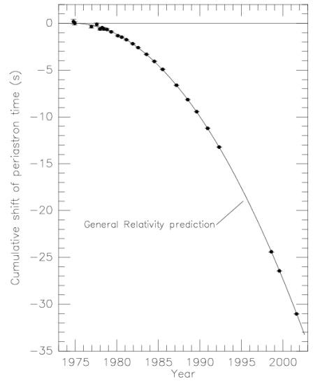
The first strong empirical evidence of gravitational waves came in 1982. The Hulse-Taylor system (section 6.2) contains two neutron stars orbiting around their common center of mass, and the period of the orbit is observed to be decreasing gradually over time (Figure 9.2.1). This is interpreted as evidence that the stars are losing energy to radiation of gravitational waves.⁴ As we’ll see later, the rate of energy loss is in excellent agreement with the predictions of general relativity.

Figure \(\PageIndex{1}\) - The Hulse-Taylor pulsar’s orbital motion is gradually losing energy due to the emission of gravitational waves. The linear decrease of the period is integrated on this plot, resulting in a parabola. From Weisberg and Taylor, http://arxiv.org/abs/astro-ph/0211217.

An even more dramatic, if less clearcut, piece of evidence is Komossa, Zhou, and Lu’s observation⁵ of a supermassive black hole that appears to be recoiling from its parent galaxy at a velocity of 2650 km/s (projected along the line of sight). They interpret this as evidence for the following scenario. In the early universe, galaxies form with supermassive black holes at their centers. When two such galaxies collide, the black holes can merge. The merger is a violent process in which intense gravitational waves are emitted, and these waves carry a large amount of momentum, causing the black holes to recoil at a velocity greater than the escape velocity of the merged galaxy.

Although the energy loss from systems such as the Hulse-Taylor binary provide strong evidence that gravitational waves exist and carry energy, physicists and astronomers still wanted to detect them directly, and serious attempts to design and build such systems began around 1962. The design that finally achieved success used interferometers which detect oscillations in the lengths of their own arms. The first gravitational-wave event was detected, by this method, in 2016, by the Advanced LIGO collaboration.⁶ The event is believed to have been the result of the collision of two black holes.

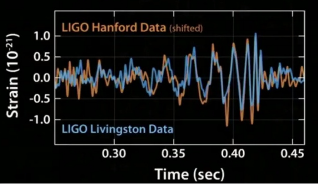
Figure \(\PageIndex{2}\) - The gravitational waveform observed in 2016 by Advanced Ligo.

In 2017, an event interpreted as the collision of two neutron stars was detected by both gravitational and electromagnetic radiation, verifying to high precision that gravitational waves propagate at c.

Although the earlier 2016 collision of black holes did not directly compare the propagation of light and gravity, it provided a different kind of check on the propagation of gravitational waves at c. The waveform detected in this event was a “chirp” that glided up in frequency as the black holes spiraled toward one another and sped up. Since the wave was in transit for over a billion years, and the waveform lasted a fraction of a second, it follows that gravitational waves within this frequency range all travel at very nearly the same velocity, i.e., there is a very tight upper limit on the dispersion of gravitational waves.

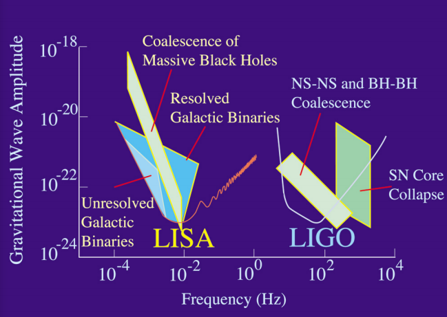
A complementary space-based system, LISA, has been proposed for launch in 2020, but its funding is uncertain. The two devices would operate in complementary frequency ranges (Figure 9.2.3). A selling point of LISA is that if it is launched, there are a number of sources in the sky, with known properties, that are known to be easily within its range of sensitivity.⁷ One excellent candidate is HM Cancri, a pair of white dwarfs with an orbital period of 5.4 minutes, shorter than that of any other known binary star.⁸

Figure \(\PageIndex{3}\) - Predicted sensitivities of LISA and LIGO to gravitational waves of various frequences.

Energy Content

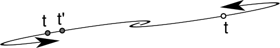
Even without performing the calculations for a system like the Hulse-Taylor binary, it is easy to show that if such waves exist, they must be capable of carrying away energy. Consider two equal masses in highly elliptical orbits about their common center of mass, Figure 9.2.4. The motion is nearly one-dimensional. As the masses recede from one another, they feel a delayed version of the gravitational force originating from a time when they were closer together and the force was stronger. The result is that in the near-Newtonian limit, they lose more kinetic and gravitational energy than they would have lost in the purely Newtonian theory. Now they come back inward in their orbits. As they approach one another, the time-delayed force is anomalously weak, so they gain less mechanical energy than expected. The result is that with each cycle, mechanical energy is lost. We expect that this energy is carried by the waves, in the same way that radio waves carry the energy lost by a transmitting antenna.⁹

Figure \(\PageIndex{4}\) - As the two planets recede from one another, each feels the gravitational attraction that the other one exerted in its previous position, delayed by the time it takes gravitational effects to propagate at c. At time t, the right-hand planet experiences the stronger deceleration corresponding to the left-hand planet’s closer position at the earlier time t', not its current position at t. Mechanical energy is not conserved, and the orbits will decay

Note

One has to be careful with this type of argument. In particular, one can obtain incorrect correct results by attempting to generalize this one-dimensional argument to motion in more than one dimension, because the effective semi-Newtonian interaction is not just a time-delayed version of Newton’s law; it also includes velocity-dependent forces. It is easy to see why such velocity-dependence must occur in the simpler case of electromagnetism. Suppose that charges A and B are not at rest relative to one another. In B’s frame, the electric field from A must come from the direction of the position that an observer comoving with B would extrapolate linearly from A’s last known position and velocity, as determined by light-speed calculation. This follows from Lorentz invariance, since this is the direction that will be seen by an observer comoving with A. A full discussion is given by Carlip, arxiv.org/abs/gr-qc/9909087v2.

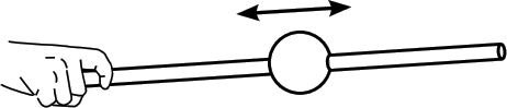
Not only can these waves remove mechanical energy from a system, they can also deposit energy in a detector, as shown by the nonmathematical “sticky bead argument” (Figure 9.2.5), which was originated by Feynman in 1957 and later popularized by Bondi.

Figure \(\PageIndex{5}\) - The sticky bead argument for the reality of gravitational waves. As a gravitational wave with the appropriate polarization passes by, the bead vibrates back and forth on the rod. Friction creates heat. This demonstrates that gravitational waves carry energy, and are thus real, observable phenomena.

Now strictly speaking, we have only shown that gravitational waves can extract or donate mechanical energy, but not that the waves themselves transmit this energy. The distinction isn’t one that normally occurs to us, since we are trained to believe that energy is always conserved. But we know that, for fundamental reasons, general relativity doesn’t have global conservation laws that apply to all spacetimes (section 4.5). Perhaps the energy lost by the Hulse-Taylor system is simply gone, never to reappear, and the energy imparted to the sticky bead is simply generated out of nowhere. On the other hand, general relativity does have global conservation laws for certain specific classes of spacetimes, including, for example, a conserved scalar mass-energy in the case of a stationary spacetime (section 7.1). Spacetimes containing gravitational waves are not stationary, but perhaps there is something similar we can do in some appropriate special case.

Suppose we want an expression for the energy of a gravitational wave in terms of its amplitude. This seems like it ought to be straightforward. We have such expressions in other classical field theories. In electromagnetism, we have energy densities +(\(\frac{1}{8 \pi k}\))|E|² and +(\(\frac{1}{2 \mu_{o}}\))|B|² associated with the electric and magnetic fields. In Newtonian gravity, we can assign an energy density −(\(\frac{1}{8 \pi G}\))|g|² to the gravitational field g; the minus sign indicates that when masses glom onto each other, they produce a greater field, and energy is released.

In general relativity, however, the equivalence principle tells us that for any gravitational field measured by one observer, we can find another observer, one who is free-falling, who says that the local field is zero. It follows that we cannot associate an energy with the curvature of a particular region of spacetime in any exact way. The best we can do is to find expressions that give the energy density (1) in the limit of weak fields, and (2) when averaged over a region of space that is large compared to the wavelength. These expressions are not unique. There are a number of ways to write them in terms of the metric and its derivatives, and they all give the same result in the appropriate limit. The reader who is interested in seeing the subject developed in detail is referred to Carroll’s Lecture Notes on General Relativity, arxiv.org/abs/gr-qc/?9712019. Although this sort of thing is technically messy, we can accomplish quite a bit simply by knowing that such results do exist, and that although they are non-unique in general, they are uniquely well defined in certain cases. Specifically, when one wants to discuss gravitational waves, it is usually possible to assume an asymptotically flat spacetime. In an asymptotically flat spacetime, there is a scalar mass-energy, called the ADM mass, that is conserved. In this restricted sense, we are assured that the books balance, and that the emission and absorption of gravitational waves really does mean the transmission of a fixed amount of energy.

Expected Properties

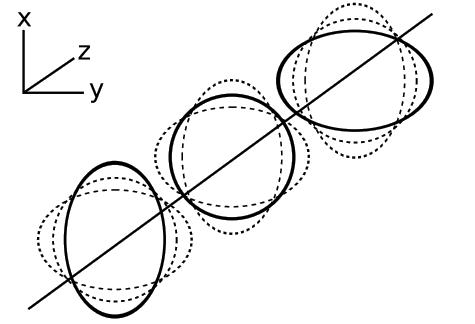
To see what properties we should expect for gravitational radiation, first consider the reasoning that led to the construction of the Ricci and Einstein tensors. If a certain volume of space is filled with test particles, then the Ricci and Einstein tensors measure the tendency for this volume to “accelerate;” i.e., \(− \frac{d^{2} V}{dt^{2}}\) is a measure of the attraction of any mass lying inside the volume. A distant mass, however, will exert only tidal forces, which distort a region without changing its volume. This suggests that as a gravitational wave passes through a certain region of space, it should distort the shape of a given region, without changing its volume.

When the idea of gravitational waves was first discussed, there was some skepticism about whether they represented an effect that was observable, even in principle. The most naive such doubt is of the same flavor as the one discussed in section 8.2 about the observability of the universe’s expansion: if everything distorts, then don’t our meter-sticks distort as well, making it impossible to measure the effect? The answer is the same as before in section 8.2; systems that are gravitationally or electromagnetically bound do not have their scales distorted by an amount equal to the change in the elements of the metric.

Figure \(\PageIndex{6}\) - As the gravitational wave propagates in the z direction, the metric oscillates in the x and y directions, preserving volume.

A less naive reason to be skeptical about gravitational waves is that just because a metric looks oscillatory, that doesn’t mean its oscillatory behavior is observable. Consider the following example.

\[ds^{2} = dt^{2} - \left(1 + \dfrac{1}{10} \sin x \right) dx^{2} - dy^{2} - dz^{2}\]

The Christoffel symbols depend on derivatives of the form \(\partial_{a} g_{bc}\), so here the only nonvanishing Christoffel symbol is \(\Gamma^{x}_{xx}\). It is then straightforward to check that the Riemann tensor

\[R^{a}_{bcd} = \partial_{c} \Gamma^{a}_{db} − \partial_{d} \Gamma^{a}_{cb} + \Gamma^{a}_{ce} \Gamma^{e}_{db} − \Gamma^{a}_{de} \Gamma^{e}_{cb}\]

vanishes by symmetry. Therefore this metric must really just be a flat-spacetime metric that has been subjected to a silly change of coordinates.

Exercise \(\PageIndex{1}\)

Self-check: R vanishes, but \(\Gamma\) doesn’t. Is there a reason for paying more attention to one or the other?

To keep the curvature from vanishing, it looks like we need a metric in which the oscillation is not restricted to a single variable.

For example, the metric

\[ds^{2} = dt^{2} - \left(1 + \frac{1}{10} \sin y \right) dx^{2} - dy^{2} - dz^{2}\]

does have nonvanishing curvature. In other words, it seems like we should be looking for transverse waves rather than longitudinal ones.¹⁰ On the other hand, this metric cannot be a solution to the vacuum field equations, since it doesn’t preserve volume. It also stands still, whereas we expect that solutions to the field equations should propagate at the velocity of light, at least for small amplitudes. These conclusions are self-consistent, because a wave’s polarization can only be constrained if it propagates at c (see section 4.2).

Note

0A more careful treatment shows that longitudinal waves can always be interpreted as physically unobservable coordinate waves, in the limit of large distances from the source. On the other hand, it is clear that no such prohibition against longitudinal waves could apply universally, because such a constraint can only be Lorentz-invariant if the wave propagates at c (see section 4.2), whereas high-amplitude waves need not propagate at c. Longitudinal waves near the source are referred to as Type III solutions in a classification scheme due to Petrov. Transverse waves, which are what we could actually observe in practical experiments, are type N.

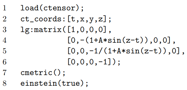
Based on what we’ve found out, the following seems like a metric that might have a fighting chance of representing a real gravitational wave:

\[ds^{2} = dt^{1} - (1 + A \sin (z - t)) dx^{2} - \frac{dy^{2}}{1 + A \sin (z - t)} - dz^{2}\]

It is transverse, it propagates at c(= 1), and the fact that g_xx is the reciprocal of g_yy makes it volume-conserving. The following Maxima program calculates its Einstein tensor:

For a representative component of the Einstein tensor, we find

\[G_{tt} = \frac{A^{2} \cos^{2} (z - t)}{2 + 4 A \sin (z - t) + 2A^{2} \sin^{2} (z - t)}\]

For small values of A, we have |G_tt| \(\lesssim \frac{A^{2}}{2}\). The vacuum field equations require G_tt = 0, so this isn’t an exact solution. But all the components of G, not just G_tt, are of order A², so this is an approximate solution to the equations.

It is also straightforward to check that propagation at approximately c was a necessary feature. For example, if we replace the factors of sin(z −t) in the metric with sin(z −2t), we get a G_xx that is of order unity, not of order A².

To prove that gravitational waves are an observable effect, we would like to be able to display a metric that (1) is an exact solution of the vacuum field equations; (2) is not merely a coordinate wave; and (3) carries momentum and energy. As late as 1936, Einstein and Rosen published a paper claiming that gravitational waves were a mathematical artifact, and did not actually exist.¹¹

References

⁴ Stairs, “Testing General Relativity with Pulsar Timing,” relativity.livingreviews.org/...es/lrr-2003-5/

⁵ http://arxiv.org/abs/0804.4585

⁶ https://dcc.ligo.org/LIGO-P150914/public

⁷ G. Nelemans, “The Galactic Gravitational wave foreground,” arxiv.org/abs/0901.1778v1

⁸ Roelofs et al., “Spectroscopic Evidence for a 5.4-Minute Orbital Period in HM Cancri,” arxiv.org/abs/1003.0658v1

¹¹ Some of the history is related at http://en.Wikipedia.org/wiki/Sticky_bead_argument.