
3.9: Thickening of a curve
- Page ID
- 13037

\( \newcommand{\vecs}[1]{\overset { \scriptstyle \rightharpoonup} {\mathbf{#1}} } \)
\( \newcommand{\vecd}[1]{\overset{-\!-\!\rightharpoonup}{\vphantom{a}\smash {#1}}} \)
\( \newcommand{\dsum}{\displaystyle\sum\limits} \)
\( \newcommand{\dint}{\displaystyle\int\limits} \)
\( \newcommand{\dlim}{\displaystyle\lim\limits} \)
\( \newcommand{\id}{\mathrm{id}}\) \( \newcommand{\Span}{\mathrm{span}}\)
( \newcommand{\kernel}{\mathrm{null}\,}\) \( \newcommand{\range}{\mathrm{range}\,}\)
\( \newcommand{\RealPart}{\mathrm{Re}}\) \( \newcommand{\ImaginaryPart}{\mathrm{Im}}\)
\( \newcommand{\Argument}{\mathrm{Arg}}\) \( \newcommand{\norm}[1]{\| #1 \|}\)
\( \newcommand{\inner}[2]{\langle #1, #2 \rangle}\)
\( \newcommand{\Span}{\mathrm{span}}\)
\( \newcommand{\id}{\mathrm{id}}\)
\( \newcommand{\Span}{\mathrm{span}}\)
\( \newcommand{\kernel}{\mathrm{null}\,}\)
\( \newcommand{\range}{\mathrm{range}\,}\)
\( \newcommand{\RealPart}{\mathrm{Re}}\)
\( \newcommand{\ImaginaryPart}{\mathrm{Im}}\)
\( \newcommand{\Argument}{\mathrm{Arg}}\)
\( \newcommand{\norm}[1]{\| #1 \|}\)
\( \newcommand{\inner}[2]{\langle #1, #2 \rangle}\)
\( \newcommand{\Span}{\mathrm{span}}\) \( \newcommand{\AA}{\unicode[.8,0]{x212B}}\)
\( \newcommand{\vectorA}[1]{\vec{#1}} % arrow\)
\( \newcommand{\vectorAt}[1]{\vec{\text{#1}}} % arrow\)
\( \newcommand{\vectorB}[1]{\overset { \scriptstyle \rightharpoonup} {\mathbf{#1}} } \)
\( \newcommand{\vectorC}[1]{\textbf{#1}} \)
\( \newcommand{\vectorD}[1]{\overrightarrow{#1}} \)
\( \newcommand{\vectorDt}[1]{\overrightarrow{\text{#1}}} \)
\( \newcommand{\vectE}[1]{\overset{-\!-\!\rightharpoonup}{\vphantom{a}\smash{\mathbf {#1}}}} \)
\( \newcommand{\vecs}[1]{\overset { \scriptstyle \rightharpoonup} {\mathbf{#1}} } \)
\(\newcommand{\longvect}{\overrightarrow}\)
\( \newcommand{\vecd}[1]{\overset{-\!-\!\rightharpoonup}{\vphantom{a}\smash {#1}}} \)
\(\newcommand{\avec}{\mathbf a}\) \(\newcommand{\bvec}{\mathbf b}\) \(\newcommand{\cvec}{\mathbf c}\) \(\newcommand{\dvec}{\mathbf d}\) \(\newcommand{\dtil}{\widetilde{\mathbf d}}\) \(\newcommand{\evec}{\mathbf e}\) \(\newcommand{\fvec}{\mathbf f}\) \(\newcommand{\nvec}{\mathbf n}\) \(\newcommand{\pvec}{\mathbf p}\) \(\newcommand{\qvec}{\mathbf q}\) \(\newcommand{\svec}{\mathbf s}\) \(\newcommand{\tvec}{\mathbf t}\) \(\newcommand{\uvec}{\mathbf u}\) \(\newcommand{\vvec}{\mathbf v}\) \(\newcommand{\wvec}{\mathbf w}\) \(\newcommand{\xvec}{\mathbf x}\) \(\newcommand{\yvec}{\mathbf y}\) \(\newcommand{\zvec}{\mathbf z}\) \(\newcommand{\rvec}{\mathbf r}\) \(\newcommand{\mvec}{\mathbf m}\) \(\newcommand{\zerovec}{\mathbf 0}\) \(\newcommand{\onevec}{\mathbf 1}\) \(\newcommand{\real}{\mathbb R}\) \(\newcommand{\twovec}[2]{\left[\begin{array}{r}#1 \\ #2 \end{array}\right]}\) \(\newcommand{\ctwovec}[2]{\left[\begin{array}{c}#1 \\ #2 \end{array}\right]}\) \(\newcommand{\threevec}[3]{\left[\begin{array}{r}#1 \\ #2 \\ #3 \end{array}\right]}\) \(\newcommand{\cthreevec}[3]{\left[\begin{array}{c}#1 \\ #2 \\ #3 \end{array}\right]}\) \(\newcommand{\fourvec}[4]{\left[\begin{array}{r}#1 \\ #2 \\ #3 \\ #4 \end{array}\right]}\) \(\newcommand{\cfourvec}[4]{\left[\begin{array}{c}#1 \\ #2 \\ #3 \\ #4 \end{array}\right]}\) \(\newcommand{\fivevec}[5]{\left[\begin{array}{r}#1 \\ #2 \\ #3 \\ #4 \\ #5 \\ \end{array}\right]}\) \(\newcommand{\cfivevec}[5]{\left[\begin{array}{c}#1 \\ #2 \\ #3 \\ #4 \\ #5 \\ \end{array}\right]}\) \(\newcommand{\mattwo}[4]{\left[\begin{array}{rr}#1 \amp #2 \\ #3 \amp #4 \\ \end{array}\right]}\) \(\newcommand{\laspan}[1]{\text{Span}\{#1\}}\) \(\newcommand{\bcal}{\cal B}\) \(\newcommand{\ccal}{\cal C}\) \(\newcommand{\scal}{\cal S}\) \(\newcommand{\wcal}{\cal W}\) \(\newcommand{\ecal}{\cal E}\) \(\newcommand{\coords}[2]{\left\{#1\right\}_{#2}}\) \(\newcommand{\gray}[1]{\color{gray}{#1}}\) \(\newcommand{\lgray}[1]{\color{lightgray}{#1}}\) \(\newcommand{\rank}{\operatorname{rank}}\) \(\newcommand{\row}{\text{Row}}\) \(\newcommand{\col}{\text{Col}}\) \(\renewcommand{\row}{\text{Row}}\) \(\newcommand{\nul}{\text{Nul}}\) \(\newcommand{\var}{\text{Var}}\) \(\newcommand{\corr}{\text{corr}}\) \(\newcommand{\len}[1]{\left|#1\right|}\) \(\newcommand{\bbar}{\overline{\bvec}}\) \(\newcommand{\bhat}{\widehat{\bvec}}\) \(\newcommand{\bperp}{\bvec^\perp}\) \(\newcommand{\xhat}{\widehat{\xvec}}\) \(\newcommand{\vhat}{\widehat{\vvec}}\) \(\newcommand{\uhat}{\widehat{\uvec}}\) \(\newcommand{\what}{\widehat{\wvec}}\) \(\newcommand{\Sighat}{\widehat{\Sigma}}\) \(\newcommand{\lt}{<}\) \(\newcommand{\gt}{>}\) \(\newcommand{\amp}{&}\) \(\definecolor{fillinmathshade}{gray}{0.9}\)Learning Objectives
- Interpret acceleration geometrically
A geometrical interpretation of the acceleration
We’ve interpreted the acceleration vector as a measure of the curvature of a world-line, but to make this more than a tool for visualization, we would have to define what we mean by curvature. A good way to approach this is shown in figure \(\PageIndex{1}\) (1).
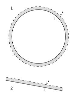
Here a circle of circumference \(L\) has been expanded, like a loaf of rising bread, to a circle of greater circumference \(L∗\). This increase is only because the circle is curved. If we do the same thing with a line segment, figure \(\PageIndex{1}\) (2), there is no increase in length. The increase in the length tells us about the curvature.
Quantitatively, suppose that the thickness of the shaded area is \(∆h\). Then the increase in circumference \(∆L = L∗ - L\) is given by
\[\frac{1}{L}\frac{\Delta L}{\Delta h} = k\]
where \(k\) is a measure of curvature, and \(k = 1/r\) for a circle. We can take this as a definition of the curvature of a curve embedded in a two-dimensional Euclidean plane. The curves in figure \(\PageIndex{1}\) (1) both have constant curvature, and if we had applied our definition to any short segment of them, we would have gotten the same answer. For a curve with varying curvature, such as a letter “\(S\),” the curvature can be defined as the appropriate limit at any given point, as the length of the segment enclosing the point approaches zero. Note that we had to pick an orientation for the expansion, i.e., a direction in which to expand. Given this orientation, it makes sense to talk about signed values of \(h\) and \(k\). If we choose the outward orientation for a circle, then its \(k\) is positive.
An interesting point about this definition is that it is extrinsic rather than intrinsic, in the sense defined in section 2.2. That is, it depends on how the curve is embedded in the ambient two-dimensional space, and it depends on the Euclidean metric of that space. Because a curve is a one-dimensional object, there is nothing internal to the curve that would allow us to define its curvature. Imagine yourself as a tiny bug — so tiny that you are pointlike. If the curve represents your universe, then you can explore it as much as you like, but you can never detect any internal evidence of its curvature. This is not the case in two dimensions. For example, a bug living on the two-dimensional surface of a sphere can detect its curvature by drawing triangles and measuring how much the sum of their interior angles differs from \(180\) degrees. This would be an intrinsic measure of curvature.
The definition given above is readily extended from Euclidean space to \(1 + 1\) dimensions of spacetime. Figure \(\PageIndex{2}\) shows a one-sided thickening of an accelerated world-line.
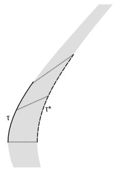
Although the shaded area doesn’t look uniformly thick to our Euclidean eyes, it is. For example, each of the dotted lines is orthogonal to the original world-line on the left, and they all have the same length \(∆h\) as measured by an observer who traces that world-line. That is, each of these lines could represent a rigid measuring rod carried by that observer, drawn along a line that that observer considers to be a line of simultaneity at that time. In analogy to the Euclidean case, we have
\[\frac{1}{\tau }\frac{\Delta \tau }{\Delta h} = \frac{1}{a}\]
Bell’s spaceship paradox
A variation on the situation shown in figure \(\PageIndex{2}\) leads to a paradox with philosophical implications proposed by John Bell. Bell went around the CERN cafeteria proposing the following thought experiment to the physicists eating lunch, and he found that nearly all of them got it wrong.
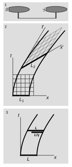
Let two spaceships accelerate as shown in figure \(\PageIndex{3}\). Each ship is equipped with a yard-arm, and a thread is tied between the two arms, figure \(\PageIndex{3}\) (1). Unaccelerated observer \(o\) uses Minkowski coordinates \((t,x)\), as shown in figure \(\PageIndex{3}\) (2). The accelerations, as judged by \(o\), are equal for the two ships as functions of \(t\). Does the thread break, due to Lorentz contraction?
A crucial difference between figures \(\PageIndex{2}\) and \(\PageIndex{3}\) (2) is that in the former, the thickening of the world-line has been carried out along the dotted normals, whereas the latter the second world-line is simply a copy of the first that has been shifted to the right, parallel to the \(x\)-axis.
The popular answer in the CERN cafeteria was that the thread would not break, the reasoning being that Lorentz contraction is a frame-dependent effect, and no such contraction would be observed in the rockets’ frames.
The error in this reasoning is that the accelerations of of the two ships were specified to be equal in frame \(o\), not in the frames of the rockets. The Minkowski coordinates \((t',x')\) shown in figure \(\PageIndex{3}\) (2) correspond to the frame of an inertial observer \(o'\) who is momentarily moving along with the trailing rocket after the acceleration has been going on for a while. The \(x'\) axis is a line of simultaneity for \(o'\), and this axis intersects the leading ship’s world-line at a point that that \(o\) considers to be later in time. Therefore \(o'\) says that the leading ship has reached a higher speed than the trailing one. In \(o'\), the two ships’ accelerations are unequal.
We can also see directly from the spacetime diagram that whereas length \(L_1\) is \(4\) units as measured by an observer initially at rest relative to the thread, \(L_2\) is about \(5\) units as measured by \(o'\), who is at rest relative to the trailing end of the thread at a later time. Since \(L_2\) is greater than the unstressed length \(L_1\), the thread is under tension.
Figure \(\PageIndex{3}\) (3) is more in the spirit of Bell’s analysis. In frame \(o\), the thread has initial, unstressed length \(L\). If the thread had been attached only to the leading ship, then it would have trailed behind it, unstressed, with Lorentz-contracted length \(L/γ\). Since its actual length according to o is still \(L\), it has been stretched relative to its unstressed length.
This paradox relates to the difficult philosophical question of whether the time dilation and length contractions predicted by relativity are “real.” This depends, of course, on what one means by “real.” They are frame-dependent, i.e., observers in different frames of reference disagree about them. But this doesn’t tell us much about their reality, since velocities are frame-dependent in Newtonian mechanics, but nobody worries about whether velocities are real. Bell took his colleagues’ wrong answers as evidence that their intuitions had been misguided by the standard way of approaching this question of the reality of Lorentz contractions.
This treatment has one wart on it, which is that we judged the distance between the two ships in a frame of reference instantaneously comoving with the trailing ship, but this is slightly different from the length as determined in the leading ship’s frame. One way to remove this wart is to note that the fractional discrepancy \(∆L_1/L_1\) is of order \(v^3\), which is of a lower order than the strain in the thread, which is of order \(v^2\). To carry out this type of error estimation rigorously would however be cumbersome. A more elegant and rigorous approach is given in section 9.5, where we use fancier techniques to show that the motion shown in figure \(\PageIndex{2}\) is the unique motion that allows every portion of the string to move without strain.
This presentation includes ideas contributed by physics forums users tiny-tim and PeterDonis.
Deja vu, jamais vu
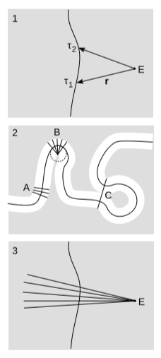
In Example 1.4.7, we saw that when an observer is accelerated, she may consider an event to be simultaneous with her more than once. That is, given a smooth, timelike world-line \(r(τ)\) parametrized by proper time, and an event \(E\), which we take to be the origin of our coordinate system, there may be more than one time at which \(r\) is orthogonal to the velocity vector \(v\) (figure \(\PageIndex{4}\) (1)). As remarked earlier, this is just a problem with applying a particular arbitrary labeling convention to a certain example — not an earthshaking crisis in physics. Nevertheless it is of some intrinsic geometric interest to characterize the circumstances under which it can happen. We would like to place some kind of bound on how much acceleration is needed and how distant E must be.
As a warm-up, consider the analogous problem in Euclidean space, figure \(\PageIndex{4}\) (2). Here we have the notion of a tubular neighborhood, which is the greatest thickening of a curve \(W\) such that no point in it lies on two different normals. The tubular neighborhood has a radius \(r\), which is the greatest possible radius of a non-self-intersecting piece of rope whose central axis coincides with \(W\). Normally, as in region \(A\), the rope doesn’t intersect itself. There are two qualitatively different reasons why the rope could self-intersect. One is local: the radius of curvature of \(W\) is too small, as at \(B\), where \(W\) coincides with a circle of radius \(r\). The other is global: two points that are far apart as measured along \(W\) could be close together in the ambient Euclidean space, as at point \(C\).
If we carry over these ideas to Minkowski space, then the local case, figure \(\PageIndex{4}\) (3), is easy to analyze using the techniques we have developed. The analog of the radius of curvature is the inverse of the proper acceleration, which suggests that we should be able to get a bound on the radius of the tubular neighborhood in terms of the acceleration. Define \(f(\tau ) = r\cdot v\). At a given point on \(W\), \(f\) is minus the Minkowski time coordinate that an observer whose world-line is \(W\) would assign, at that instant, to \(E\). The condition for the type of self-intersection we’re discussing is that both \(f\) and its derivative with respect to proper time \(f'\) vanish at the same point on \(W\). Differentiating f using the product rule, we find \(f' = v\cdot v + r\cdot a = 1 + r\cdot a\) (in the \(+---\) signature), so that \(r\cdot a = -1\).
We now make use of the fact that both \(a\) and \(r\) are orthogonal to \(W\) — the former as a general kinematic fact, and the latter because \(f = 0\). This means that they lie in the plane perpendicular to \(W\). The geometry of this plane is Euclidean, so we can apply the Euclidean inequality \(|a \cdot r| \leq |a| |r|\), where the bars on the left denote the absolute value and the ones on the right the magnitudes of the vectors. We therefore have \(|a| |r| \geq 1\). Since \(r\) is orthogonal to \(W\), we can interpret it as the proper distance between \(E\) and \(W\). The magnitude of \(a\) is the proper acceleration. Converting to units with \(c \neq 1\), we have an exact bound of the form \(\text{(proper distance)(proper acceleration)}\geq c^2\). In ordinary units \(c\) is large, so in this sense \(E\) must be distant, and the acceleration large. This explains why we never encounter such a problem in nonrelativistic physics.
That was never now
So far we have characterized the circumstances under which simultaneity can fail to be unique. Simultaneity can also fail to exist. For example, in the same notation, take \(W\) to be the constant acceleration motion described in Example 3.5.1, and let \(E\) be the event \((-1,0)\). Then it can easily be shown that \(f(τ)\) is always positive, so an observer moving along \(W\) will always consider \(E\) to be in her past, never her future. No time exists for her such that she considers \(E\) to be “now.” The function \(f\) comes to a maximum somewhere but never crosses zero.
There will always be some neighborhood of \(W\) within which we are protected against nonexistence of simultaneity. To determine the radius of this neighborhood, we consider an event \(B\) that lies on the boundary of the neighborhood, and define \(f\) in terms of \(B\) rather than \(E\). Then \(f(τ) = 0\) for some \(τ\), but \(f\) does not cross over zero, so that either \(f \leq 0\) everywhere or \(f \geq 0\) everywhere. At the place where \(f(τ) = 0\), we also have \(f'(τ) = 0\), and the rest of the analysis is the same as before. Therefore the radius of the tubular neighborhood determined in that example defines a radius within which simultaneity has both existence and uniqueness.
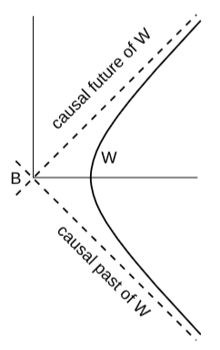
The interpretation of such a boundary point \(B\) is a little funny. Figure \(\PageIndex{5}\) recapitulates the motion described in Example 3.5.1. For this motion, the only point like \(B\) is the one labeled \((0,0)\) in the Minkowski coordinates used in that derivation. Is there really anything special about this point, or is it just a random point that we happened to choose as the origin of our coordinate system? An observer moving along this \(W\) does not believe that any point in spacetime accessible to her has any special properties. She has always been accelerating and always will be, so no event she can observe or affect can be distinguished from the other events that she could have observed or affected in the same way at any earlier or later time. But we can easily show that \(B\) is special by giving a description of it without reference to any coordinates. Let \(W\)’s causal future be the set of all events that lie in the future light cone of some event on \(W\), and similarly for \(W\)’s causal past. The boundaries of these two sets are \(W\)’s past and future event horizons, and these horizons coincide at only one event, which is \(B\). This seems paradoxical, but our observer can neither observe nor affect \(B\), so there is no contradiction.