7.3: Transformation of the Metric

Learning Objectives

• Explain the transformation of the metric when we change from Minkowski coordinates

Continuing with the example of accelerated coordinates, let’s find what happens to the metric when we change from Minkowski coordinates. Minkowski coordinates are essentially defined so that the metric has the familiar form with coefficients $+1$ and $-1$. In relativity, one often presents the metric by showing its result when applied to an infinitesimal displacement $(dt,dx)$:

$$ds^2 = dt^2 - dx^2$$

Here $ds$ would represent proper time, in the case where the displacement was timelike. Since we’ve already determined that

$$dt = X \cosh T dT + \sinh T dX$$

and

$$dx = X \sinh T dT + \cosh T dX$$

we can simply substitute into the expression for ds in order to find the form of the metric in $(T,X)$ coordinates. Employing the identity $\cosh ^2 - \sinh ^2 = 1$, we find

$$ds^2 = X^2 dT^2 - dX^2$$

The varying value of the $dT^2$ coefficient is in fact exactly the kind of gravitational time dilation effect whose existence we predicted in section 5.2 based on the equivalence principle. The form of the metric inferred there was

$$ds^2 ≈ (1 + 2∆Φ) dT^2 - dX^2$$

where $∆Φ$ is the difference in gravitational potential relative to some reference height. One of the approximations employed was the assumption that the range of heights $X$ was small, but subject to that approximation, the two results should agree. For convenience, let’s consider observers in the region $X ≈ 1$, where the acceleration is approximately $1$. Then the $∆Φ = Φ(1 + ∆X) - Φ(1) ≈ \text{(acceleration)(height)} ≈ X$, so the time coefficient in the second form of the metric is $≈ 1+2∆Φ ≈ 1+2∆X$. But to within the desired level of approximation, this is the same as $X^2 = (1+∆X)^2 ≈ 1 + 2∆X$.

The procedure employed above works in general. To transform the metric from coordinates $(t,x,y,z)$ to new coordinates $(t',x',y',z')$, we obtain the unprimed coordinates in terms of the primed ones, take differentials on both sides, and eliminate $t, ..., dt, ...$ in favor of $t', ...dt', ...$ in the expression for $ds^2$. We’ll see in section 9.2, that this is an example of a more general transformation law for tensors, mathematical objects that generalize vectors and covectors in the same way that matrices generalize row and column vectors. A scalar, with no indices, is called a tensor of rank $0$. Vectors and covectors, having one index, are called rank-$1$ tensors.

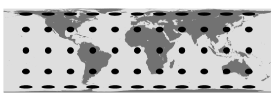
Example $\PageIndex{1}$: A map projection

Because the earth’s surface is curved, it is not possible to represent it on a flat map without distortion. Let $φ$ be the latitude, θ the angle measured down from the north pole (known as the colatitude), both measured in radians, and let a be the earth’s radius. Then by the definition of radian measure, an infinitesimal north-south displacement by $dθ$ is a distance $adθ$. A point at a given colatitude $θ$ lies at a distance $a \sinθ$ from the axis, so for an infinitesimal east-west distance we have $a \sin θ dφ$. For convenience, let the units be chosen such that $a = 1$. Then the metric, with signature $++$, is

$$ds^2 = dθ^2 +\sin^2 θ dφ$$

One of the many possible ways of forming a flat map is the Lambert cylindrical projection,

$$x = φ$$

$$y = \cosθ$$

is shown in figure $\PageIndex{1}$. If we see a distance on the map and want to know how far it actually is on the earth’s surface, we need

to transform the metric into the $(x,y)$ coordinates. The inverse coordinate transformation is

$$φ = x$$

$$θ = \cos^{-1} y$$

Taking differentials on both sides, we get

$$dφ = dx$$

$$d\theta = -\dfrac{dy}{\sqrt{1-y^2}}$$

We take the metric and eliminate $θ$, $φ$, $dθ$, and $dφ$, finding

$$ds^2 = (1 - y^2)dx^2 + \dfrac{1}{1 - y^2}dy^2$$

In Fgure $\PageIndex{1}$, the polka-dot pattern is made of figures that are actually circles, all of equal size, on the earth’s surface. Since they are fairly small, we can approximate $y$ as having a single value for each circle, which means that they are represented on the flat map as approximate ellipses with their east-west dimensions having been stretched by $(1 - y^2)^{-1/2}$ and their north-south ones shrunk by $(1 - y^2)^{1/2}$. Since these two factors are reciprocals of one another, the area of each ellipse is the same as the area of the original circle, and therefore the same as those of all the other ellipses. They are a visual representation of the metric, and they demonstrate the equal-area property of this projection.

Figure $\PageIndex{1}$: The polka-dot pattern is made of figures that are actually circles, all of equal size, on the earth’s surface.