9.3: Gauss’s Theorem

Learning Objectives

• Explain simple and general form of Gauss's theorem

Integral Conservation Laws

We’ve expressed conservation of charge and energy-momentum in terms of zero divergences,

$$\frac{\partial J^a}{\partial x^a} = 0$$

$$\frac{\partial T^{ab}}{\partial x^a} = 0$$

These are expressed in terms of derivatives. The derivative of a function at a certain point only depends on the behavior of the function near that point, so these are local statements of conservation. Conservation laws can also be stated globally: the total amount of something remains constant. Taking charge as an example, observer $o$ defines Minkowski coordinates $(t, x, y, z)$, and at a time t1 says that the total amount of charge in some region is

$$q(t_1) = \int_{t_1}J^a dS_a$$

where the subscript $t_1$ means that the integrand is to be evaluated over the surface of simultaneity $t = t_1$, and $dS_a = (dx dy dz, 0, 0, 0)$ is an element of $3$-volume expressed as a covector. The charge at some later time $t_2$ would be given by a similar integral. If charge is conserved, and if our region is surrounded by an empty region through which no charge is coming in or out, then we should have $q(t_2) = q(t_1)$.

A simple form of Gauss’s theorem

The connection between the local and global conservation laws is provided by a theorem called Gauss’s theorem. In your course on electromagnetism, you learned Gauss’s law, which relates the electric flux through a closed surface to the charge contained inside the surface. In the case where no charges are present, it says that the flux through such a surface cancels out.

Figure $\PageIndex{1}$: Three lines go in, and three come out. These could be field lines or world lines.

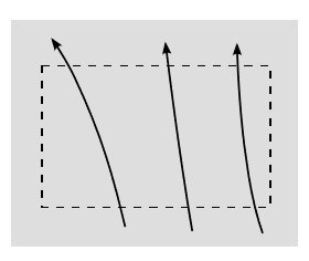
The interpretation is that since field lines only begin or end on charges, the absence of any charges means that the lines can’t begin or end, and therefore, as in figure $\PageIndex{1}$, any field line that enters the surface (contributing some negative flux) must eventually come back out (creating some positive flux that cancels out the negative). But there is nothing about figure $\PageIndex{1}$ that requires it to be interpreted as a drawing of electric field lines. It could just as easily be a drawing of the worldlines of some charged particles in $1 + 1$ dimensions. The bottom of the rectangle would then be the surface at $t_1$ and the top $t_2$. We have $q(t_1) = 3$ and $q(t_2) = 3$ as well.

For simplicity, let’s start with a very restricted version of Gauss’s theorem. Let a vector field $J^a$ be defined in two dimensions. (We don’t care whether the two dimensions are both spacelike or one spacelike and one timelike; that is, Gauss’s theorem doesn’t depend on the signature of the metric.) Let $R$ be a rectangular area, and let $S$ be its boundary. Define the flux of the field through $S$ as

$$\Phi = \int_{S}J^a dS_a$$

where the integral is to be taken over all four sides, and the covector $dS_a$ points outward. If the field has zero divergence, $\frac{\partial J^a}{\partial x^a} = 0$, then the flux is zero.

Proof: Define coordinates $x$ and $y$ aligned with the rectangle. Along the top of the rectangle, the element of the surface, oriented outwards, is $dS = (0, dx)$, so the contribution to the flux from the top is

$$\Phi _{top} = \int_{top}J^y (y_{top}) dx$$

At the bottom, an outward orientation gives $dS = (0, -dx)$, so

$$\Phi _{bottom} = \int_{bottom}J^y (y_{bottom}) dx$$

Using the fundamental theorem of calculus, the sum of these is

$$\Phi _{top} + \Phi _{bottom} = \int_{R}\frac{\partial J^y}{\partial y}dy dx$$

Adding in the similar expressions for the left and right, we get

$$\Phi = \int_{R}\left (\frac{\partial J^x}{\partial x} + \frac{\partial J^y}{\partial y} \right )dy dx$$

But the integrand is the divergence, which is zero by assumption, so $Φ = 0$ as claimed.

The general form of Gauss’s theorem

Although the coordinates were labeled $x$ and $y$, the proof made no use of the metric, so the result is equally valid regardless of the signature. The rectangle could equally well have been a rectangle in $1 + 1$-dimensional spacetime. The generalization to $n$ dimensions is also automatic, and everything also carries through without modification if we replace the vector $J^a$ with a tensor such as $T^{ab}$ that has more indices — the extra index $b$ just comes along for the ride. Sometimes, as with Gauss’s law in electromagnetism, we are interested in fields whose divergences are not zero. Gauss’s theorem then becomes

$$\int_{S} J^a dS_a= \int_{R}\frac{\partial J^a}{\partial x^a} dv$$

where $dv$ is the element of $n$-volume. In $3 + 1$ dimensions we could use Minkowski coordinates to write the element of $4$-volume as $dv = dt dx dy dz$, and even though this expression in written in terms of these specific coordinates, it is actually Lorentz invariant ( section 2.5).

Figure $\PageIndex{2}$: Proof of Gauss’s theorem for a region with an arbitrary shape.

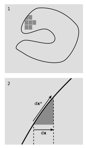
The generalization to a region $R$ with an arbitrary shape, figure $\PageIndex{2}$, is less trivial. The basic idea is to break up the region into rectanglular boxes, figure $\PageIndex{2}$ (1). Where the faces of two boxes coincide on the interior of $R$, their own outward directions are opposite. Therefore if we add up the fluxes through the surfaces of all the boxes, the contributions on the interior cancel, and we’re left with only the exterior contributions. If $R$ could be dissected exactly into boxes, then this would complete the proof, since the sum of exterior contributions would be the same as the flux through $S$, and the left-hand side of Gauss’s theorem would be additive over the boxes, as is the right-hand side.

The difficulty arises because a smooth shape typically cannot be built out of bricks, a fact that is well known to Lego enthusiasts who build elaborate models of the Death Star. We could argue on physical grounds that no real-world measurement of the flux can depend on the granular structure of $S$ at arbitrarily small scales, but this feels a little unsatisfying. For comparison, it is not strictly true that surface areas can be treated in this way. For example, if we approximate a unit $3$-sphere using smaller and smaller boxes, the limit of the surface area is $6π$, which is quite a bit greater than the surface area $4π/3$ of the limiting surface.

Instead, we explicitly consider the nonrectangular pieces at the surface, such as the one in figure $\PageIndex{2}$ (2). In this drawing in $n = 2$ dimensions, the top of this piece is approximately a line, and in the limit we’ll be considering, where its width becomes an infinitesimally small $dx$, the error incurred by approximating it as a line will be negligible. We define vectors $dx$ and $dx ∗$ as shown in the figure. In more than the two dimensions shown in the figure, we would approximate the top surface as an $(n - 1)$-dimensional parallelepiped spanned by vectors $dx ∗ , dy ∗ , . . .$ This is the point at which the use of the covector $S_a$ pays off by greatly simplifying the proof.¹ Applying this to the top of the triangle, $dS$ is defined as the linear function that takes a vector $J$ and gives the $n$-volume spanned by $J$ along with $dx ∗ , . . .$

Call the vertical coordinate on the diagram $t$, and consider the contribution to the flux from $J$’s time component, $J^t$. Because the triangle’s size is an infinitesimal of order $dx$, we can approximate $J^t$ as being a constant throughout the triangle, while incurring only an error of order $dx$. (By stating Gauss’s theorem in terms of derivatives of $J$, we implicitly assumed it to be differentiable, so it is not possible for it to jump discontinuously.) Since $dS$ depends linearly not just on $J$ but on all the vectors, the difference between the flux at the top and bottom of the triangle equals is proportional to the area spanned by $J$ and $dx ∗ - dx$. But the latter vector is in the $t$ direction, and therefore the area it spans when taken with $J^t$ is approximately zero. Therefore the contribution of $J^t$ to the flux through the triangle is zero. To estimate the possible error due to the approximations, we have to count powers of $dx$. The possible variation of $J^t$ over the triangle is of order $(dx)^1$. The covector $dS$ is of order $(dx)^{n-1}$, so the possible error in the flux is of order $(dx)^n$.

This was only an estimate of one part of the flux, the part contributed by the component $J^t$. However, we get the same estimate for the other parts. For example, if we refer to the two dimensions in figure $\PageIndex{1}$ (2) as $t$ and $x$, then interchanging the roles of $t$ and $x$ in the above argument produces the same error estimate for the contribution from $J^x$.

This is good. When we began this argument, we were motivated to be cautious by our observation that a quantity such as the surface area of $R$ can’t be calculated as the limit of the surface area as approximated using boxes. The reason we have that problem for surface area is that the error in the approximation on a small patch is of order $(dx)^{n-1}$, which is an infinitesimal of the same order as the surface area of the patch itself. Therefore when we scale down the boxes, the error doesn’t get small compared to the total area. But when we consider flux, the error contibuted by each of the irregularly shaped pieces near the surface goes like $(dx)^n$, which is of the order of the $n$-volume of the piece. This volume goes to zero in the limit where the boxes get small, and therefore the error goes to zero as well. This establishes the generalization of Gauss’s theorem to a region $R$ of arbitrary shape.

9.3.4 The energy-momentum vector

Einstein’s celebrated $E = mc^2$ is a special case of the statement that energy-momentum is conserved, transforms like a four-vector, and has a norm $m$ equal to the rest mass. Section 4.4 explored some of the problems with Einstein’s original attempt at a proof of this statement, but only now are we prepared to completely resolve them. One of the problems was the definitional one of what we mean by the energy-momentum of a system that is not composed of pointlike particles. The answer is that for any phenomenon that carries energy-momentum, we must decide how it contributes to the stress-energy tensor. For example, the stress-energy tensor of the electric and magnetic fields is described in section 10.6.

Figure $\PageIndex{3}$: Conservation of the integrated energy-momentum vector.

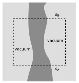
For the reasons discussed in Section 4.4, it is necessary to assume that energy-momentum is locally conserved, and also that the system being described is isolated. Local conservation is described by the zero-divergence property of the stress-energy tensor, $\frac{\partial T^{ab}}{\partial x^a} = 0$. Once we assume local conservation, figure $\PageIndex{3}$ shows how to prove conservation of the integrated energy-momentum vector using Gauss’s theorem. Fix a frame of reference $o$. Surrounding the system, shown as a dark stream flowing through spacetime, we draw a box. The box is bounded on its past side by a surface that $o$ considers to be a surface of simultaneity $s_A$, and likewise on the future side $s_B$. It doesn’t actually matter if the sides of the box are straight or curved according to o. What does matter is that because the system is isolated, we have enough room so that between the system and the sides of the box there can be a region of vacuum, in which the stress-energy tensor vanishes. Observer $o$ says that at the initial time corresponding to $s_A$, the total amount of energy-momentum in the system was

$$p_{A}^{\mu } = -\int_{s_A} T^{\mu \nu } dS_{\nu }$$

where the minus sign occurs because we take $dS_{\nu }$ to point outward, for compatibility with Gauss’s theorem, and this makes it antiparallel to the velocity vector $o$, which is the opposite of the orientation defined in equations 9.2.1 and 9.2.2. At the final time we have

$$p_{B}^{\mu } = \int_{s_B} T^{\mu \nu } dS_{\nu }$$

with a plus sign because the outward direction is now the same as the direction of $o$. Because of the vacuum region, there is no flux through the sides of the box, and therefore by Gauss’s theorem

$$p_{B}^{\mu } - p_{A}^{\mu } = 0$$

The energy-momentum vector has been globally conserved according to $o$.

Figure $\PageIndex{4}$: Lorentz transformation of the integrated energy-momentum vector.

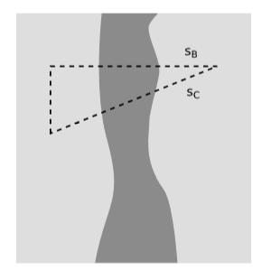
We also need to show that the integrated energy-momentum transforms properly as a four-vector. To prove this, we apply Gauss’s theorem to the region shown in figure $\PageIndex{4}$, where $s_C$ is a surface of simultaneity according to some other observer $o'$. Gauss’s theorem tells us that $p_B = p_C$, which means that the energy-momentum on the two surfaces is the same vector in the absolute sense — but this doesn’t mean that the two vectors have the same components as measured by different observers. Observer $o$ says that $s_B$ is a surface of simultaneity, and therefore considers $p_B$ to be the total energy-momentum at a certain time. She says the total mass-energy is $p_{B}^{\mu } o_{\mu }$ (Equation 9.2.1), and similarly for the total momentum in the three spatial directions $s_1$, $s_2$, and $s_3$ (Equation 9.2.2). Observer $o'$, meanwhile, considers $s_C$ to be a surface of simultaneity, and has the same interpretations for quantities such as $p_{C}^{\mu } o'_{\mu }$. But this is just a way of saying that $p_{B}^{\mu }$ and $p_{C}^{\mu }$ are related to each other by a change of basis from $(o, s_1, s_2, s_3)$ to $(o', s'_1, s'_2, s'_3)$. A change of basis like this is just what we mean by a Lorentz transformation, so the integrated energy-momentum $p$ transforms as a four-vector.

9.3.5 Angular momentum

In section 8.2, we gave physical and mathematical plausibility arguments for defining relativistic angular momentum as $L^{ab} = r^a p^b - r^b p^a$. We can now show that this quantity is actually conserved. Just as the flux of energy-momentum $p^a$ is the stress-energy tensor $T^{ab}$, we can take the angular momentum $L^{ab}$ and define its flux $λ^{abc} = r^a T^{bc} - r^b T^{ac}$. An observer with velocity vector $o^c$ says that the density of energy-momentum is $T^{ac}o_c$ and the density of angular momentum is $λ^{abc}o_c$. If we can show that the divergence of $λ$ with respect to its third index is zero, then it follows that angular momentum is conserved. The divergence is

$$\frac{\partial \lambda ^{abc}}{\partial x^c} = \frac{\partial }{\partial x^c} \left (r^a T^{bc} - r^b T^{ac} \right )$$

The product rule gives

$$\frac{\partial \lambda ^{abc}}{\partial x^c} = \delta _{c}^{a} T^{bc} + r^a \frac{\partial }{\partial x^c} T^{bc} - \delta _{c}^{b} T^{ac} - r^b \frac{\partial }{\partial x^c} T^{ac}$$

where $\delta _{j}^{i}$, called the Kronecker delta, is defined as $1$ if $i = j$ and $0$ if $i \neq j$. The divergence of the stress-energy tensor is zero, so the second and fourth terms vanish, and

$$\begin{align*} \frac{\partial \lambda ^{abc}}{\partial x^c} &= \delta _{c}^{a} T^{bc} - \delta _{c}^{b} T^{ac}\\ &= T^{ba} - T^{ab} \end{align*}$$

but this is zero because the stress-energy tensor is symmetric.

References

¹ Here is an example of the ugly complications that occur if one doesn’t have access to this piece of technology. In the low-tech approach, in Euclidean space, one defines an element of surface area $dA = \hat{n} dA$, where the unit vector $\hat {n}$ is outward-directed with $\hat{n} \cdot \hat{n} = 1$. But in a signature such as +−−−, we could have a region $R$ such that over some large area of the bounding surface $S$, the normal direction was lightlike. It would therefore be impossible to scale $\hat {n}$ so that $\hat{n} \cdot \hat{n}$ was anything but zero. As an example of how much work it is to resolve such issues using stone-age tools, see Synge, Relativity: The Special Theory, VIII, §6-7, where the complete argument takes up 22 pages.