9.1: The Current Vector

Learning Objectives

• Explain the conservation of charge

Current as the flux of charged particles

The most fundamental laws of physics are conservation laws, which tell us that we can’t create or destroy “stuff,” where “stuff” could mean quantities such as electric charge or energy-momentum. Since charge is a Lorentz invariant, it’s an easy example to start with. Because charge is invariant, we might also imagine that charge density \(ρ\) was invariant. But this is not the case, essentially because spatial (\(3\)-dimensional) volume isn’t invariant; in \(3 + 1\) dimensions, only four -dimensional volume is an invariant . For example, suppose we have an insulator in the shape of a cube, with charge distributed uniformly throughout it according to an observer \(o_1\) at rest relative to the cube. Then in a frame \(o_2\) moving relative to the cube, parallel to one of its axes, the cube becomes foreshortened by length contraction, and its volume is reduced by the factor \(1/γ\). The result is that the charge density in \(o_2\) is greater by a factor of \(γ\).

This means that knowledge of the charge density \(ρ\) in one frame is insufficient to determine the charge density in another frame. In the example of the cube, what would be sufficient would be knowledge of the vector \(J = ρ_0 v\), where \(ρ_0\) is the charge density in the cube’s rest frame, and \(v\) is the cube’s velocity vector. \(J\), called the current vector, transforms as a relativistic vector because of the transformation properties of the two factors that define it. The velocity \(v\) is a vector (section 3.5). The factor \(ρ_0\) is an invariant, since it in turn breaks down into charge divided by rest-volume. Charge is an invariant, and all observers agree on what the volume the cube would have in its rest frame.

Figure \(\PageIndex{1}\): Charged particles with world-lines that contribute to \(J_x\) and \(ρ\). The \(z\) dimension isn’t shown, so the cubical 3-surfaces appear as squares.

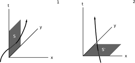
\(J\) can be expressed in Minkowski coordinates as \((ρ, J^x, J^y, J^z)\), where \(ρ\) is the charge density and, e.g., \(J^x\) is the density of electric current in the \(x\) direction. Suppose we define the three-surface \(S\) shown in figure \(\PageIndex{1}\) (1), consisting of the set of events with coordinates \((t, 0, y, z)\) such that \(0 ≤ t ≤ 1\), \(0 ≤ y ≤ 1\), and \(0 ≤ z ≤ 1\). Some charged particles have world-lines that intersect this surface, passing through it either in the positive \(x\) direction or the negative \(x\) direction (which we count as negative charge transport). \(S\) has a three-volume \(V\). If we add up the total charge transport \(∆q\) across this surface and divide by \(V\), we get the average value of \(J^x\). If we let \(S\) shrink down to smaller and smaller three-surfaces surrounding the event \((0, 0, 0, 0)\), then we get the the value of \(J^x\) at this point, \(lim_{V\to 0} \frac{\Delta q}{V}\). In other words, \(J^x\) measures the flux density of charge that passes through \(S\). Of course this description in terms of a limit implies a large number of charges, not just one as in figure \(\PageIndex{1}\).

You can write out the analogous definition for \(J^t\), using a surface of simultaneity for like \(S'\), figure \(\PageIndex{1}\) (2), and you’ll see that it expresses the density of charge \(ρ\). In this case \(S'\) represents a moment in time, and the flux through \(S'\) means that the charges are crossing the threshold from the past into the future.

Our argument that \(J\) transformed like a vector was based on a case where all the charged particles had the same velocity vector, but the above description in terms of the flux of charge eliminated any discussion of velocity. It’s true, but less obvious, that the \(J\) described in this way also transforms as a vector, even in cases where the charged particles do not all have parallel world-lines. The current vector is the source of electric and magnetic fields. Remarkably, no macroscopic electrical measurement is capable of detecting anything more detailed about the motion of the charges than the averaged information provided by \(J\).

Example \(\PageIndex{1}\): Boosting a solenoid

Figure \(\PageIndex{2}\): Solenoid

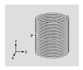
The figure \(\PageIndex{2}\) shows a solenoid, at rest, wound from copper wire. At point \(P\), we construct a rectangular Ampérian loop in the \(yz\) plane that has its right edge inside the solenoid and its left one outside. Ampére’s law,

\[\int B\cdot ds = \left ( \frac{4\pi k}{c^2} \right )l\]

then tells us that the current density \(J_x\) causes a difference between the exterior field \(B_z = 0\) and the interior field \(B_z = \left ( \frac{4\pi k}{c^2} \right )J_x \Delta y\), where \(∆y\) is the thickness of the solenoid. There are two things we can get from this result, both of them nontrivial.

First, the field depends only on the current density, not on any information about the details of the motion of the electrons in the copper. The electrons’ motion is fast and highly random, but all that contributes to \(J_x\) is the slow drift velocity, typically \(∼ 1\: cm/s\), superimposed on the randomness. This is exact and not at all obvious. For example, the total momentum of the electrons does depend on the random part of their motion, because \(p_x = mγv_x\) has a factor of \(γ\) in it.

Second, we can use the transformation properties of the current vector to find the field of this solenoid in a frame boosted along its axis. This is the kind of situation that would naturally arise, for example, in an electric motor whose rotor contains an electromagnet. A Lorentz transformation in the \(z\) direction doesn’t change the \(x\) component of a vector, nor does it change \(∆y\), so \(B_z\) is the same in both frames. This is nontrivial both in the sense that it would have been difficult to figure out by brute force and in the sense that fields don’t have to be the same in different frames of reference — for example, a boost in the \(x\) or the \(y\) direction would have changed the result.

Example \(\PageIndex{2}\): A wire

In a solid conductor such as a copper wire, we have two types of charges, protons and electrons. The protons are at rest in the lab frame \(o\), with charge density \(ρ_p\) and current density

\[J_p = (ρ_p, 0, 0, 0) \]

in Minkowski coordinates. The motion of the electrons is complicated. Some electrons are bound to a particular atom, but still move at relativistic speeds within their atoms. Others exhibit violent thermal motion that very nearly, but not quite, averages out to zero when there is a current measurable by an ammeter. For simplicity, we treat all the electrons (both the bound ones and the mobile ones) as a single density of charge \(ρ_e\). Let the average velocity of the electrons, known as their drift velocity, be \(v\) in the \(x\) direction. Then in the frame \(o'\) moving along with the drift velocity we have

\[J_{e}^{'} = (\rho _{e}^{'}, 0, 0, 0)\]

which under a Lorentz transformation back into the lab frame becomes

\[J_{e} = (\rho _{e}^{'}\gamma , \rho _{e}^{'}V\gamma , 0, 0)\]

Adding the two current vectors, we have a total current in the lab frame

\[J = (\rho _p + \rho _{e}^{'}\gamma , \rho _{e}^{'}V\gamma , 0, 0)\]

The wire is electrically neutral in this frame, so \(\rho _p + \rho _{e}^{'}\gamma =0\). Since \(ρ_p\) is a fixed property of the wire, we express \(\rho _{e}^{'}\) in terms of it as \(ρ_p/γ\). Eliminating \(\rho _{e}^{'}\) gives

\[J = (0, -ρ_pV, 0, 0)\]

Because the \(γ\) factors canceled, we find that the current is exactly proportional to the drift velocity. Geometrically, we have added two timelike vectors and gotten a spacelike one; this is possible because one of the timelike vectors was future-directed and the other past-directed.

Conservation of charge

Figure \(\PageIndex{3}\):

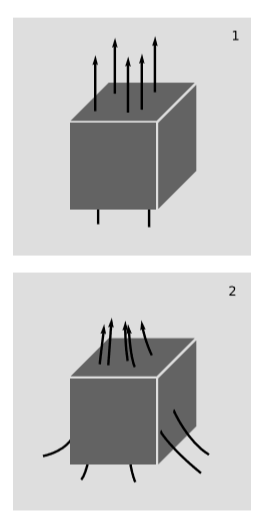
Conservation of charge can be expressed elegantly in terms of \(J\). Charge density is the timelike component \(J^t\). If this charge density near a certain point is, for example, increasing, then it might be because charge conservation has been violated as in figure \(\PageIndex{3}\) (1). In this example, more world-lines emerge into the future at the top of the four-cube than had entered through the bottom in the past. Some process inside the cube is creating charge. In the limit where the cube is made very small, this would be measured by a value of \(\frac{\partial J^t}{\partial t}\) that was greater than zero.

But experiments have never detected any violation of charge conservation, so if more charge is emerging from the top (future) side of the cube than came in from the bottom (past), the more likely explanation is that the charges are not all at rest, as in figure \(\PageIndex{3}\) (1), but are moving, figure \(\PageIndex{3}\) (2), and there has been a net flow in from neighboring regions of space. We should find this reflected in the spatial components \(J^x\), \(J^y\) and \(J^z\). Moreover, if these spatial components were all constant, then any given region of space would have just as much current flowing into it from one side as there was flowing out the other. We therefore need to have some nonzero partial derivatives such as \(\frac{\partial J^x}{\partial x}\). For example, figure \(\PageIndex{3}\) (2)has a positive \(J^x\) on the left and a negative \(J^x\) on the right, so \(\frac{\partial J^x}{\partial x} < 0\). Charge conservation is expressed by the simple equation \(\frac{\partial J^{\lambda }}{\partial x^{\lambda }} = 0\). Writing out the implied sum over \(λ\), this says that

\[\frac{\partial J^t}{\partial t} + \frac{\partial J^x}{\partial x} + \frac{\partial J^y}{\partial y} + \frac{\partial J^z}{\partial z} = 0\]

with an implied sum over the index \(λ\). If you’ve taken vector calculus, you’ll recognize the operator being applied to \(J\) as a four-dimensional generalization of the divergence. This charge-conservation equation is valid regardless of the coordinate system, so it can also be rewritten in abstract index notation as

\[\frac{\partial J^a}{\partial x^a} = 0\]

Example \(\PageIndex{3}\): Conservation of charge in a solenoid

In a solenoid, we have charge circulating at some drift velocity \(v\). Ignoring the protons, and adapting the relevant expression from example \(\PageIndex{2}\) to the case of circular rather than linear motion, we might have for the electrons’ contribution to the current something of the form

\[J = p(1, -qy, qx, 0),\]

where \(p = γv\) and \(q\) depends on the \(v\) and on the radius of the solenoid. Conservation of charge is satisfied, because each of the four terms in the equation

\[\frac{\partial J^t}{\partial t} + \frac{\partial J^x}{\partial x} + \frac{\partial J^y}{\partial y} + \frac{\partial J^z}{\partial z} = 0\]

vanishes individually.