2.6: Qualitative Features of Entropy

The concept of entropy is notoriously difficult to grasp. Even the consummate mathematician and physicist Johnny von Neumann claimed that “nobody really knows what entropy is anyway.” Although we have an exact and remarkably simple formula for the entropy of a macrostate in terms of the number of corresponding microstates, this simplicity merely hides the subtle characterization needed for a real understanding of the entropy concept. To gain that understanding, we must examine the truly wonderful (in the original meaning of that overused word) surprises that this simple formula presents when applied to real physical systems.

Surprises

The monatomic ideal gas

Let us examine the Sackur-Tetrode formula (2.32) qualitatively to see whether it agrees with our understanding of entropy as proportional to the number of microstates corresponding to a given macrostate. If the volume \(V\) is increased, then the formula states that the entropy \(S\) increases, which certainly seems reasonable: If the volume goes up, then each particle has more places where it can be, so the entropy ought to increase. If the energy \(E\) is increased, then \(S\) increases, which again seems reasonable: If there is more energy around, then there will be more different ways to split it up and share it among the particles, so we expect the entropy to increase. (Just as there are many more ways to distribute a large booty among a certain number of pirates than there are to distribute a small booty.) But what if the mass m of each particle increases? (Experimentally, one could compare the entropy of, say, argon and krypton under identical conditions. See problem 2.27.) Our formula shows that entropy increases with mass, but is there any way to understand this qualitatively?

In fact, I can produce not just one but two qualitative arguments concerning the dependence of \(S\) on \(m\). Unfortunately the two arguments give opposite results! The first relies upon the fact that

\[E=\frac{1}{2 m} \sum_{i} p_{i}^{2},\]

so for a given energy \(E\), any individual particle may have a momentum ranging from 0 to \( \sqrt{2mE}\). A larger mass implies a wider range of possible momenta, which suggests more microstates and a greater entropy. The second argument relies upon the fact that

\[E=\frac{m}{2} \sum_{i} v_{i}^{2},\]

so for a given energy \(E\), any individual particle may have a speed ranging from 0 to \( \sqrt{E/m}\). A larger mass implies a narrowed range of possible speeds, which suggests fewer microstates and a smaller entropy. The moral is simple: Qualitative arguments can backfire!

That’s the moral of the paradox. The resolution of the paradox is both deeper and more subtle: It hinges on the fact that the proper home of statistical mechanics is phase space, not configuration space, because Liouville’s theorem implies conservation of volume in phase space, not in configuration space. This issue deeply worried the founders of statistical mechanics. See Ludwig Boltzmann, Vorlesungen über Gastheorie (J.A. Barth, Leipzig, 1896–98), part II, chapters III and VII [translated into English by Stephen G. Brush: Lectures on Gas Theory (University of California Press, Berkeley, 1964)]; J. Willard Gibbs, Elementary Principles in Statistical Mechanics (C. Scribner’s Sons, New York, 1902), page 3; and Richard C. Tolman, The Principles of Statistical Mechanics (Oxford University Press, Oxford, U.K., 1938), pages 45, 51–52.

Freezing water

It is common to hear entropy associated with “disorder,” “smoothness,” or “homogeneity.” How do these associations stand up to the simple situation of a bowl of liquid water placed into a freezer? Initially the water is smooth and homogeneous. As its temperature falls, the sample remains homogeneous until the freezing point is reached. At the freezing temperature the sample is an inhomogeneous mixture of ice and liquid water until all the liquid freezes. Then the sample is homogeneous again as the temperature continues to fall. Thus the sample has passed from homogeneous to inhomogeneous to homogeneous, yet all the while its entropy has decreased. (We will see later that the entropy of a sample always decreases as its temperature falls.)

Suppose the ice is then cracked out of its bowl to make slivers, which are placed back into the bowl and allowed to rest at room temperature until they melt. The jumble of irregular ice slivers certainly seems disordered relative to the homogeneous bowl of meltwater, yet it is the ice slivers that have the lower entropy. The moral here is that the huge number of microscopic degrees of freedom in the meltwater completely overshadow the minute number of macroscopic degrees of freedom in the jumbled ice slivers. But the analogies of entropy to “disorder” or “smoothness” invite us to ignore this moral and concentrate on the system’s gross appearance and nearly irrelevant macroscopic features.

Reentrant phases

When the temperature falls at constant pressure, most pure materials pass from gas to liquid to solid. But the unusual materials called “liquid crystals,” which consist of rod-like molecules, display a larger number of phases. For typical liquid crystals, the high-temperature liquid phase is isotropic, meaning that the positions and the orientations of the molecules are scattered about nearly at random. At lower temperatures, the substance undergoes a transition into the so-called “nematic” phase, in which the molecules tend to orient

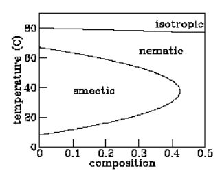
Figure \(\PageIndex{1}\): Phase diagram of a liquid crystal mixture. The variable “composition” refers to the molecular weight ratio of 6OCB to 8OCB.

in the same direction but in which positions are still scattered. At still lower temperatures it passes into the “smectic” phase, in which the molecules orient in the same direction and their positions tend to fall into planes. Finally, at even lower temperatures, the molecules freeze into a conventional solid. The story told so far reinforces the picture of “entropy as disorder,” with lower-temperature (hence lower entropy) phases showing more and more qualitative order.

But not all liquid crystals behave in exactly this fashion. One material called “hexyloxy-cyanobiphenyl” or “6OCB” passes from isotropic liquid to nematic to smectic and then back to nematic again as the temperature is lowered. The first transition suggests that the nematic phase is “less orderly” than the smectic phase, while the second transition suggests the opposite!

One might argue that the lower-temperature nematic phase — the so-called “reentrant nematic” — is somehow qualitatively different in character from the higher-temperature nematic, but the experiments summarized in figure \(\PageIndex{1}\) demonstrate that this is not the case. These experiments involve a similar liquid crystal material called “octyloxy-cyanobiphenyl” or “8OCB” which has no smectic phase at all. Adding a bit of \(\text{8OCB}\) into a sample of \(\text{6OCB}\) reduces the temperature range over which the smectic phase exists. Adding a bit more reduces that range further. Finally, addition of enough \(\text{8OCB}\) makes the smectic phase disappear altogether. The implication of figure \(\PageIndex{1}\) is clear: there is no qualitative difference between the usual nematic and the reentrant nematic phases — you can move continuously from one to the other in the temperature–composition phase diagram.

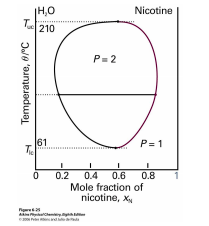
Figure \(\PageIndex{2}\): Phase diagram for a mixture of water and nicotine.

The implication of reentrant phases for entropy is profound: Under some conditions the nematic phase has more entropy than the smectic phase and under other conditions less, while in all cases the nematic is qualitatively less ordered. Another example of reentrant behavior appears in the phase diagram of the mixture of water and nicotine (see figure \(\PageIndex{2}\)). For a wide range of mixing ratios, this mixture is a homogeneous solution at high temperatures, segregates into water-rich and nicotine-rich phases at moderate temperatures, yet becomes homogeneous again at low temperatures. At mixing ratios closer to pure water or pure nicotine, the mixture is homogeneous at all temperatures. Thus the high-temperature and reentrant homogeneous phases are in fact the same phase. (Reentrant phases are also encountered in type-II superconductors.)

Rust

According to a common misconception, “The entropy law describes the tendency for all objects to rust, break, fall apart, wear out, and otherwise move to a less ordered state.”⁶ Or “Entropy tends to make our eyes grow weaker as we age . . . entropy causes iron and other metals to rust.”⁷ Or “Entropy imposes itself in the form of limitation and in the natural tendency toward confusion and chaos, toward decay and destruction. Entropy is why ice cream melts and people die. It is why cars rust and forests burn. Preponderantly, the second law describes effects that we don’t want to see.”⁸

At least one error is held in common by these three quotes. Does rusting lead to increased entropy?

The rust reaction is

\[\text{4 Fe } + \text{ 3 O}_2 \to \text{ 2 Fe}_2\text{O}_3.\]

According to standard tables⁹ the entropy (at room temperature \(\text{298.15 K}\) and at pressure \(\text{105 Pa}\)) of one mole of \(\text{Fe}\) is \(\text{27.280 J/K}\), of one mole of \(\text{O}_2\) is \(\text{205.147 J/K}\), and of one mole of \(\text{Fe}_2\text{O}_3\) is \(\text{87.404 J/K}\). The entropy of the reactants is \(\text{724.561 J/K}\), the entropy of the products is \(\text{174.808 J/K}\), so the reaction results in an entropy decrease of \(\text{549.753 J/K}\).

It is easy to understand why this should be so: gases typically have much greater entropies that solids. And of course this doesn’t mean that during rusting, the entropy of the universe decreases: although the entropy of the iron plus oxygen decreases, the entropy of the surroundings increases by even more. Nevertheless, it is clear that rusting itself involves a decrease in entropy, not an increase.

Entropy and the lattice gas

The four examples above should caution us about relying on qualitative arguments concerning entropy. Here is another situation¹⁰ to challenge your intuition: The next page shows two configurations of \(132 = 169\) squares tossed down on an area that has \(35 \times 35 = 1225\) empty spaces, each of which could hold a square. (This system is called the “lattice gas model.”) The two configurations were produced by two different computer programs (Toss1 and Toss2 ) that used different rules to position the squares. (The rules will be presented in due course; for the moment I shall reveal only that both rules employ random numbers.) Which configuration do you think has the greater entropy? Be sure look at the configurations, ponder, and make a guess (no matter how ill-informed) before reading on.

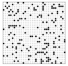
Figure \(\PageIndex{3}\): A lattice gas configuration generated by the program Toss1.

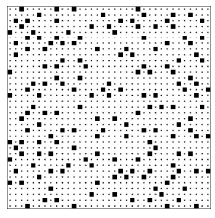
Figure \(\PageIndex{4}\): A lattice gas configuration generated by the program Toss2.

Before analyzing these pictures, I must first confess that my question was very misleading. I asked “Which configuration has the greater entropy?”, but entropy is not defined in terms of a single configuration (a single microstate). Instead, entropy is defined for a macrostate, and is related to the number of microstates that the system can take on and still be classified in that same macrostate. Instead of asking the question I did, I should have pointed out that I had two classes, two pools, of microstates, and that I used my two computer programs to select one member from each of those two pools. The selection was done at random, so the selected configuration should be considered typical. Thus my question should have been “Which configuration was drawn from the larger pool?”, or “Which configuration is typical of the larger class?”. Given this corrected question, you might want to go back and look at the configurations again.

I have asked these questions of a number of people (both students and professionals) and most of them guess that the lower configuration (the output of program Toss2), is typical of the class with larger entropy. The lower configuration is smoother, less clumpy. They look at the upper configuration and see patterns, which suggests some orderly process for producing that configuration, while the smoothness of the lower configuration suggests a random, disorderly construction process. Let me end the suspense and tell you how my computer programs produced the two configurations. The top configuration was produced by tossing \(169 = (13)^2\) squares down at random onto an area with \(35 \times 35 = 1225\) locations, subject only to the rule that two squares could not fall on the same location. The bottom configuration was produced in exactly the same manner except that there was an additional rule, namely that two squares could not fall on adjacent locations either. Thus the top configuration was drawn from the pool of all patterns with 169 squares, while the bottom configuration was drawn from the much smaller pool of patterns with 169 squares and with no two squares adjacent. The top configuration is typical of the class with more configurations and hence greater entropy.

Look again at the bottom configuration. You will notice that there are no squares immediately adjacent to any given square. This “nearest neighbor exclusion” rule acts to spread out the squares, giving rise to the smooth appearance that tricks so many into guessing that the bottom configuration is typical of a class with high entropy.

Now look again at the top configuration. You will notice holes and clumps of squares, the inhomogeneities that lead many to guess that it is typical of a small class. But in fact one should expect a random configuration to have holes — only a very exceptional configuration is perfectly smooth.¹¹ This involves the distinction between a typical configuration and an average configuration. Typical configurations have holes: some have holes in the upper right, some in the middle left, some in the very center. Because the holes fall in various locations, the average configuration — the one produced by adding all the configurations and dividing by the number of configurations — is smooth. The average configuration is actually atypical. (Analogy: A typical person is not of average height. A typical person is somewhat taller or somewhat shorter than average, and very few people are exactly of average height. Any clothing manufacturer that produced only shirts of average size would quickly go bankrupt.) The presence of holes or clumps, therefore, need not be an indication of a pattern or of a design. However, we humans tend to find patterns wherever we look, even when no design is present.¹² In just this way the ancient Greeks looked into the nighttime sky, with stars sprinkled about at random, and saw the animals, gods, and heroes that became our constellations.

Entropy and poker

An excellent illustration of the nature of entropy is given by the card game poker. There are many possible hands in poker, some valuable and most less so. For example, the hand

\[A♥, K♥, Q♥, J♥, 10♥\]

is an example of a royal flush, the most powerful hand in poker. There are only four royal flushes (the royal flush of hearts, of diamonds, of spades, and of clubs) and any poker player who has ever been dealt a royal flush will remember it for the rest of his life.

By contrast, no one can remember whether he has been dealt the hand

\[4♦, 3♦, J♥, 2♠, 7♦\]

because this hand is a member of an enormous class of not-particularly-valuable poker hands. But the probability of being dealt this hand is exactly the same as the probability of being dealt the royal flush of hearts. The reason that one hand is memorable and the other is not has nothing to do with the rarity of that particular hand, it has everything to do with the size of the class of which the hand is a member.

This illustration of the importance of class rather than individual configuration is so powerful and so graphic that I shall call that distinction “the poker paradox”.

Conclusion

It is often said that entropy is a measure of the disorder of a system. This qualitative concept has at least three failings: First, it is vague. There is no precise definition of disorder. Some find the abstract paintings of Jackson Pollock to be disorderly; others find them pregnant with structure. Second, it uses an emotionally charged word. Most of us have feelings about disorder (either for it or against it), and the analogy encourages us to transfer that like or dislike from disorder, where our feelings are appropriate, to entropy, where they are not. The most important failing, however, is that the analogy between entropy and disorder invites us to think about a single configuration rather than a class of configurations. In the lattice gas model there are many “orderly” configurations (such as the checkerboard pattern of figure 2.6) that are members of both classes. There are many other “orderly” configurations (such as the solid block pattern of figure \(\PageIndex{6}\)) that are members only of the larger (higher entropy!) class.¹³ The poker hand

\[2♣, 4♦, 6♥, 8♠, 10♣\]

is very orderly, but a member of a very large class of nearly worthless poker hands.

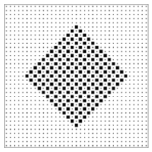
Figure \(\PageIndex{5}\): An orderly lattice gas configuration that is a member of both the large class and the small class of configurations.

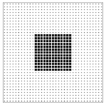
Figure \(\PageIndex{6}\): An orderly lattice gas configuration that is a member of only the large (high entropy!) class of configurations.

Given the clear need for an intuition concerning entropy, and the appealing but unsatisfactory character of the simile “entropy as disorder,” what is to be done? I suggest an additional simile, namely “entropy as freedom,” which should be used not by itself but in conjunction with “entropy as disorder.”

“Freedom” means a range of possible actions, while “entropy” means a range of possible microstates. If only one microstate corresponds to a certain macrostate, then the system has no freedom to choose its microstate — and it has zero entropy. If you are free to manage your own bedroom, then you may keep it either neat or messy, just as high entropy macrostates encompass both orderly and disorderly microstates. The entropy gives the number of ways that the constituents of a system can be arranged and still be a member of the club (or class). If the class entropy is high, then there are a number of different ways to satisfy the class membership criteria. If the class entropy is low, then that class is very demanding — very restrictive — about which microstates it will admit as members. In short, the advantage of the “entropy as freedom” analogy is that it focuses attention on the variety of microstates corresponding to a macrostate whereas the “entropy as disorder” analogy invites focus on a single microstate.

While “entropy as freedom” has these benefits, it also has two of the drawbacks of “entropy as disorder.” First, the term “freedom” is laden with even more emotional baggage than the term “disorder.” Second, it is even more vague: political movements from the far right through the center to the extreme left all characterize themselves as “freedom fighters.” Is there any way to reap the benefits of this analogy without sinking into the mire of drawbacks?

For maximum advantage, I suggest using both of these analogies. The emotions and vaguenesses attached to “freedom” are very different from those attached to “disorder,” so using them together tends to cancel out the emotion. A simple sentence like “For macrostates of high entropy, the system has the freedom to chose one of a large number of microstates, and the bulk of such microstates are microscopically disordered” directs attention away from glib emotional baggage and toward the perspective of “more entropy means more microstates.”

But perhaps it is even better to avoid analogies all together. Just think of entropy as describing the number of microstates consistent with the prescribed macrostate. And then you will remember always that entropy applies to a macrostate, i.e. a class of microstates, rather than to an individual microstate.

Problems

2.17 Entropy of the classical monatomic ideal gas: limits

a. Every macrostate has at least one corresponding microstate. Use this to show that in all cases \(S \geq 0\).

b. Use the Sackur-Tetrode formula (2.31) to find the entropy of the classical monatomic ideal gas in the limit of high density (i.e. volume per particle approaches zero). [This absurd result indicates a breakdown in the approximation of “ideal” non-interacting particles. At high densities, as the particles crowd together, it is no longer possible to ignore the repulsive interactions which are responsible for the “size” of each atom.]

c. What is the entropy of the classical monatomic ideal gas when the energy equals the ground-state energy (i.e. \(E \to 0\))? [This absurd result indicates a breakdown in the “classical” approximation. As we will see in chapter 6, quantum mechanics becomes a significant effect at low energies. Historically, this absurdity was one of the first indications that classical mechanics could not be universally true.]

2.18 (Q,E) The coin toss

If you flip a coin ten times, you expect on average to get five heads and five tails.

a. The pattern HHHHHHHHHH violates this expectation dramatically. What is the probability of obtaining this pattern?

b. The pattern HTHTHTHTHT matches this expectation exactly. What is the probability of obtaining this pattern?

c. What is the probability of obtaining the pattern HTTTHHTTHT?

d. What is the probability of obtaining a pattern with one tail and nine heads?

2.19 (Q) Random walks

You are presented with two pictures that supposedly sketch the progress of a random walker as it moves through space. One was drawn by a computer using a random number generator, the other by a human being. One picture is more or less uniform, the other has some spaces dark with lines and other spaces hardly touched. Which picture was drawn in which way?

2.20 Poker

In the game of poker, a hand consists of five cards drawn from a deck of 52 cards. The cards are evenly divided into four suits (hearts, diamonds, clubs, spades).

a. How many hands are there in poker? Explain your reasoning.

b. How many hands are flushes? (That is, all five cards of the same suit.)

c. Harry plays poker every evening, and each evening he is dealt 100 hands. How long must Harry play, on average, before being dealt the hand

\[4♦, 3♦, J♥, 2♠, 7♦\]

⁶Cutler J. Cleveland and Robert Kaufmann “Fundamental principles of energy,” in Encyclopedia of Earth, last updated 29 August 2008, http://www.eoearth.org/article/Fundamental-principles-of-energy.

⁷Louis M. Savary, Teilhard de Chardin: The Divine Milieu Explained (Paulist Press, Mahwah, NJ, 2007) page 163.

⁸Gilbert L. Wedekind, Spiritual Entropy (Xulon Press, Fairfax, VA, 2003) page 68.

⁹Ihsan Barin, Thermochemical Data of Pure Substances (VCH Publishers, Weinheim, Germany, 1995) pages 675, 1239, and 702.

¹⁰The argument of this section was invented by Edward M. Purcell and is summarized in Stephen Jay Gould, Bully for Brontosaurus (W.W. Norton, New York, 1991), pages 265–268, 260–261. The computer programs mentioned, which work under MS-DOS, are available for free downloading through http://www.oberlin.edu/physics/dstyer/.

¹¹In his book The Second Law (Scientific American Books, New York, 1984), P.W. Atkins promotes the idea that entropy is a measure of homogeneity. (This despite the everyday observation of two-phase coexistence.) To buttress this argument, the book presents six illustrations (on pages 54, 72, 74, 75, and 77) of “equilibrium lattice gas configurations.” Each configuration has 100 occupied sites on a \(40 \times 40\) grid. If the occupied sites had been selected at random, then the probability of any site being occupied would be \(100/1600\), and the probability of any given pair of sites both being occupied would be \(1/(16)^2\). The array contains \(2 \times 39 \times 39\) adjacent site pairs, so the expected number of occupied adjacent pairs would be \(2(39/16)^ = 11.88\). The actual numbers of occupied nearest-neighbor pairs in the six illustrations are \(0, 7, 3, 7, 4\), and \(3\). A similar calculation shows that the expected number of empty rows or columns in a randomly occupied array is \((15/16)10 \times 2 \times 40 = 41.96\). The actual numbers for the six illustrations are \(28, 5, 5, 4, 4\), and \(0\). I am confident that the sites in these illustrations were not occupied at random, but rather to give the impression of uniformity.

¹²Look again at figure \(\PageIndex{3}\). Do you see the dog catching a ball in the middle left? Do you see the starship Enterprise in the bottom right?

¹³Someone might raise the objection: “Yes, but how many configurations would you have to draw from the pool, on average, before you obtained exactly the special configuration of figure \(\PageIndex{6}\)?” The answer is, “Precisely the same number that you would need to draw, on average, before you obtained exactly the special configuration of figure \(\PageIndex{3}\).” These two configurations are equally special and equally rare.