
3.4: Multivariate Calculus
- Page ID
- 6346

\( \newcommand{\vecs}[1]{\overset { \scriptstyle \rightharpoonup} {\mathbf{#1}} } \)
\( \newcommand{\vecd}[1]{\overset{-\!-\!\rightharpoonup}{\vphantom{a}\smash {#1}}} \)
\( \newcommand{\dsum}{\displaystyle\sum\limits} \)
\( \newcommand{\dint}{\displaystyle\int\limits} \)
\( \newcommand{\dlim}{\displaystyle\lim\limits} \)
\( \newcommand{\id}{\mathrm{id}}\) \( \newcommand{\Span}{\mathrm{span}}\)
( \newcommand{\kernel}{\mathrm{null}\,}\) \( \newcommand{\range}{\mathrm{range}\,}\)
\( \newcommand{\RealPart}{\mathrm{Re}}\) \( \newcommand{\ImaginaryPart}{\mathrm{Im}}\)
\( \newcommand{\Argument}{\mathrm{Arg}}\) \( \newcommand{\norm}[1]{\| #1 \|}\)
\( \newcommand{\inner}[2]{\langle #1, #2 \rangle}\)
\( \newcommand{\Span}{\mathrm{span}}\)
\( \newcommand{\id}{\mathrm{id}}\)
\( \newcommand{\Span}{\mathrm{span}}\)
\( \newcommand{\kernel}{\mathrm{null}\,}\)
\( \newcommand{\range}{\mathrm{range}\,}\)
\( \newcommand{\RealPart}{\mathrm{Re}}\)
\( \newcommand{\ImaginaryPart}{\mathrm{Im}}\)
\( \newcommand{\Argument}{\mathrm{Arg}}\)
\( \newcommand{\norm}[1]{\| #1 \|}\)
\( \newcommand{\inner}[2]{\langle #1, #2 \rangle}\)
\( \newcommand{\Span}{\mathrm{span}}\) \( \newcommand{\AA}{\unicode[.8,0]{x212B}}\)
\( \newcommand{\vectorA}[1]{\vec{#1}} % arrow\)
\( \newcommand{\vectorAt}[1]{\vec{\text{#1}}} % arrow\)
\( \newcommand{\vectorB}[1]{\overset { \scriptstyle \rightharpoonup} {\mathbf{#1}} } \)
\( \newcommand{\vectorC}[1]{\textbf{#1}} \)
\( \newcommand{\vectorD}[1]{\overrightarrow{#1}} \)
\( \newcommand{\vectorDt}[1]{\overrightarrow{\text{#1}}} \)
\( \newcommand{\vectE}[1]{\overset{-\!-\!\rightharpoonup}{\vphantom{a}\smash{\mathbf {#1}}}} \)
\( \newcommand{\vecs}[1]{\overset { \scriptstyle \rightharpoonup} {\mathbf{#1}} } \)
\(\newcommand{\longvect}{\overrightarrow}\)
\( \newcommand{\vecd}[1]{\overset{-\!-\!\rightharpoonup}{\vphantom{a}\smash {#1}}} \)
\(\newcommand{\avec}{\mathbf a}\) \(\newcommand{\bvec}{\mathbf b}\) \(\newcommand{\cvec}{\mathbf c}\) \(\newcommand{\dvec}{\mathbf d}\) \(\newcommand{\dtil}{\widetilde{\mathbf d}}\) \(\newcommand{\evec}{\mathbf e}\) \(\newcommand{\fvec}{\mathbf f}\) \(\newcommand{\nvec}{\mathbf n}\) \(\newcommand{\pvec}{\mathbf p}\) \(\newcommand{\qvec}{\mathbf q}\) \(\newcommand{\svec}{\mathbf s}\) \(\newcommand{\tvec}{\mathbf t}\) \(\newcommand{\uvec}{\mathbf u}\) \(\newcommand{\vvec}{\mathbf v}\) \(\newcommand{\wvec}{\mathbf w}\) \(\newcommand{\xvec}{\mathbf x}\) \(\newcommand{\yvec}{\mathbf y}\) \(\newcommand{\zvec}{\mathbf z}\) \(\newcommand{\rvec}{\mathbf r}\) \(\newcommand{\mvec}{\mathbf m}\) \(\newcommand{\zerovec}{\mathbf 0}\) \(\newcommand{\onevec}{\mathbf 1}\) \(\newcommand{\real}{\mathbb R}\) \(\newcommand{\twovec}[2]{\left[\begin{array}{r}#1 \\ #2 \end{array}\right]}\) \(\newcommand{\ctwovec}[2]{\left[\begin{array}{c}#1 \\ #2 \end{array}\right]}\) \(\newcommand{\threevec}[3]{\left[\begin{array}{r}#1 \\ #2 \\ #3 \end{array}\right]}\) \(\newcommand{\cthreevec}[3]{\left[\begin{array}{c}#1 \\ #2 \\ #3 \end{array}\right]}\) \(\newcommand{\fourvec}[4]{\left[\begin{array}{r}#1 \\ #2 \\ #3 \\ #4 \end{array}\right]}\) \(\newcommand{\cfourvec}[4]{\left[\begin{array}{c}#1 \\ #2 \\ #3 \\ #4 \end{array}\right]}\) \(\newcommand{\fivevec}[5]{\left[\begin{array}{r}#1 \\ #2 \\ #3 \\ #4 \\ #5 \\ \end{array}\right]}\) \(\newcommand{\cfivevec}[5]{\left[\begin{array}{c}#1 \\ #2 \\ #3 \\ #4 \\ #5 \\ \end{array}\right]}\) \(\newcommand{\mattwo}[4]{\left[\begin{array}{rr}#1 \amp #2 \\ #3 \amp #4 \\ \end{array}\right]}\) \(\newcommand{\laspan}[1]{\text{Span}\{#1\}}\) \(\newcommand{\bcal}{\cal B}\) \(\newcommand{\ccal}{\cal C}\) \(\newcommand{\scal}{\cal S}\) \(\newcommand{\wcal}{\cal W}\) \(\newcommand{\ecal}{\cal E}\) \(\newcommand{\coords}[2]{\left\{#1\right\}_{#2}}\) \(\newcommand{\gray}[1]{\color{gray}{#1}}\) \(\newcommand{\lgray}[1]{\color{lightgray}{#1}}\) \(\newcommand{\rank}{\operatorname{rank}}\) \(\newcommand{\row}{\text{Row}}\) \(\newcommand{\col}{\text{Col}}\) \(\renewcommand{\row}{\text{Row}}\) \(\newcommand{\nul}{\text{Nul}}\) \(\newcommand{\var}{\text{Var}}\) \(\newcommand{\corr}{\text{corr}}\) \(\newcommand{\len}[1]{\left|#1\right|}\) \(\newcommand{\bbar}{\overline{\bvec}}\) \(\newcommand{\bhat}{\widehat{\bvec}}\) \(\newcommand{\bperp}{\bvec^\perp}\) \(\newcommand{\xhat}{\widehat{\xvec}}\) \(\newcommand{\vhat}{\widehat{\vvec}}\) \(\newcommand{\uhat}{\widehat{\uvec}}\) \(\newcommand{\what}{\widehat{\wvec}}\) \(\newcommand{\Sighat}{\widehat{\Sigma}}\) \(\newcommand{\lt}{<}\) \(\newcommand{\gt}{>}\) \(\newcommand{\amp}{&}\) \(\definecolor{fillinmathshade}{gray}{0.9}\)What is a section on multivariate calculus doing in a physics book. . . particularly a physics book which assumes that you already know multivariate calculus? The answer is that you went through your multivariate calculus course learning one topic after another, and there are some subtle topics that you covered early in the course that really couldn’t be properly understood until you had covered other topics that came later in the course. (This is not the fault of your teacher in multivariate calculus, because the later topics could not be understood at all without an exposure to the earlier topics.) This section goes back and investigates five subtle points from multivariate calculus to make sure they don’t trip you when they are applied to thermodynamics.
3.4.1 What is a partial derivative?
Given a function f(x, y, z), what is the meaning of ∂f/∂y? Many will answer that
\[\frac{\partial f}{\partial y} \text { is the change of } f \text { with } y \text { while everything else is held constant. }\]
This answer is WRONG! If f changes, then f2 changes, and sin(f) changes, and so forth, so it can’t be that “everything else” is held constant. The proper answer is that
\[\frac{\partial f}{\partial y} \text { is the change of } f \text { with } y \text { while all other variables are held constant. }\]
Thus it becomes essential to keep clear which quantities are variables and which are functions. This is not usually hard in the context of mathematics: the functions are f, g, and h while the variables are x, y, and z. But in the context of physics we use symbols like E, V, p, T, and N which suggest the quantities they represent, and it is easy to mix up the functions and the variables.
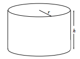
An illustration from geometry makes this point very well. Consider the set of all right circular cylinders. Each cylinder can be specified uniquely by the variables r, radius, and h, height. If you know r and h for a cylinder you can readily calculate any quantity of interest—such as the area of the top, T(r, h), the area of the side S(r, h), and the volume V(r, h)—as shown on the left side of the table below. But this is not the only way to specify each cylinder uniquely. For example, if you know the height and the side area of the cylinder, you may readily calculate the radius and hence find our previous specification. Indeed, the specification through the variables S and h is just as good as the one through the variables r and h, as is shown on the right side of the table below. [There are many other possible specifications (e.g. r and S, or T and V) but these two sets will be sufficient to make our point.]
Describing a Cylinder
\( \begin{array}{cl}{\textbf{ variables: }} & {\textbf{ variables: }} \\ {\text { radius } r} & {\text { side area } S} \\ {\text { height } h} & {\text { height } h} \\ {\textbf{ functions: }} & {\textbf{ functions: }} \\ {\text { top area } T(r, h)=\pi r^{2}} & {\text { radius } r(S, h)=S / 2 \pi h} \\ {\text { side area } S(r, h)=2 \pi r h} & {\text { top area } T(S, h)=S^{2} / 4 \pi h^{2}} \\ {\text { volume } V(r, h)=\pi r^{2} h} & {\text { volume } V(S, h)=S^{2} / 4 \pi h}\end{array}\)
All of this is quite straightforward and ordinary. But now we ask one more question concerning the geometry of cylinders, namely “How does the volume change with height?” The last line of the table presents two formulas for volume, so taking appropriate derivative gives us either
\[\frac{\partial V}{\partial h}=\pi r^{2}=T \quad \text { or } \quad \frac{\partial V}{\partial h}=-S^{2} / 4 \pi h^{2}=-T.\]
What? Is ∂V/∂h equal to T or to −T? It can’t be equal to both! The problem with equation (3.11) is that we were careless about specifying the variables. The two expressions for volume,
\[V(r, h)=\pi r^{2} h \quad \text { and } \quad V(S, h)=S^{2} / 4 \pi h,\]
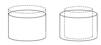
are in fact two completely different functions, with completely different variables, so we should expect completely different derivatives. If we increase the height h keeping the radius r fixed, the figure on the left below makes it clear that the volume increases. But if we increase the height and keep the side area S fixed, the radius will have to decrease as shown on the right below. The change on the right adds to the volume at the top of the cylinder but subtracts from the volume all along the sides. It would be most remarkable if the two volume changes were equal and, as our derivatives have shown, they are not.
A mathematician would say that we got ourselves in trouble in equation (3.11) because we gave two different functions the same name. A physicist would reply that they both represent the volume, so they deserve the same name. Rather than get into an argument, it is best to write out the variables of all functions explicitly, thus rewriting (3.11) as
\[\frac{\partial V(r, h)}{\partial h}=\pi r^{2}=T(r, h) \quad \text { or } \quad \frac{\partial V(S, h)}{\partial h}=-S^{2} / 4 \pi h^{2}=-T(S, h).\]
(Physicists often neglect to write out the full list of variables, which saves some time and some ink but which invites error. R.H. Price and J.D. Romano (Am. J. Phys. 66 (1998) 114) expose a situation in which a physicist published a deep error, which he made by neglecting to write out an explicit variable list.)
It becomes tiresome to write out the entire argument list for every function, so a shorthand notation has been developed. A right hand parenthesis is written after the partial derivative, and the functional arguments that are not being differentiated are listed as subscripts to that parenthesis. Thus the derivatives above are written as
\[\frac{\partial V(r, h)}{\partial h}=\frac{\partial V}{\partial h} )_{r} \quad \text { and } \quad \frac{\partial V(S, h)}{\partial h}=\frac{\partial V}{\partial h} )_{S}.\]
The expression on the left is read “the partial derivative of V with respect to h while r is held constant”.
3.4.2 The Legendre transformation
Let us return to a description of cylinders in terms of the variables r and h. Clearly, one of the functions of interest is the volume
\[V (r, h).\]
A glance at the table on page 58 (or a moment’s thought about geometry) shows that the total differential of V as a function of r and h is
\[d V=S(r, h) d r+T(r, h) d h,\]
whence
\[S(r, h)=\frac{\partial V}{\partial r} )_{h} \quad \text { and } \quad T(r, h)=\frac{\partial V}{\partial h} )_{r}.\]
Thus knowledge of the function V(r, h) gives us a bonus. . . if we know V(r, h), then we can take simple derivatives to find the other quantities of interest concerning cylinders, namely S(r, h) and T(r, h). Because of the central importance of V (r, h), it is called a “master function” and the total differential (3.16) is called a “master equation”.
Is there any way to find a similarly convenient “master description” in terms of the variables S and h? Indeed there is, and it is given by the “Legendre transformation”. In the Legendre transformation from the variables r and h to the variables S and h, we change the focus of our attention from the master function V(r, h) to the function
\[\Phi(S, h)=V(r(S, h), h)-S r(S, h).\]
(The above equation is written out in full with all arguments shown. It is more usually seen as
\[\Phi=V-S r,\]
although this form raises the possibility that variables and functions will become mixed up.) The total differential of Φ is
\[d \Phi =d V-S d r-r d S\]
\[ =S d r+T d h-S d r-r d S\]
\[ =-r d S+T d h\]
We have found a new master function! It is
\[\Phi(S, h),\]
and the new master equation is
\[d \Phi=-r(S, h) d S+T(S, h) d h,\]
giving rise immediately to
\[r(S, h)=-\frac{\partial \Phi}{\partial S} )_{h} \quad \text { and } \quad T(S, h)=\frac{\partial \Phi}{\partial h} )_{S}.\]
This description has all the characteristics of a master description: once the master function is known, all the other interesting functions can be found by taking straightforward derivatives.
3.4.3 Maxwell relations
Suppose
\[df = A(x, y) dx + B(x, y) dy. (3.26)\]
Then
\(A(x, y)=\frac{\partial f}{\partial x} )_{y} \quad \text { and } \quad B(x, y)=\frac{\partial f}{\partial y} )_{x}.\)
But because
\(\frac{\partial^{2} f(x, y)}{\partial x \partial y}=\frac{\partial^{2} f(x, y)}{\partial y \partial x}\)
it follows that
\[\frac{\partial A}{\partial y} )_{x}=\frac{\partial B}{\partial x} )_{y}.\]
This is called a "Maxwell relation".
Applied to equation (3.16), this tells us at a glance that
\[\frac{\partial S}{\partial h} )_{r}=\frac{\partial T}{\partial r} )_{h}.\]
We know that these two derivatives are equal without needing to find either one of them! Applied to equation (3.24), it tells us with equal ease that
\[ \frac{\partial r}{\partial h} )_{S}=-\frac{\partial T}{\partial S} )_{h}.\]
3.4.4 Implicit function theorem
Suppose f(x, y) is a function of the variables x and y. What is
\[\frac{\partial y}{\partial x} )_{f}\]
the slope of a contour of constant f?
Start with
\[d f=\frac{\partial f}{\partial x} )_{y} d x+\frac{\partial f}{\partial y} )_{x} d y.\]
which holds for any differential change dx and dy. But we’re not interested in any differential change: to evaluate the slope (3.30), we need a change in which df = 0 so
\( 0=\frac{\partial f}{\partial x} )_{y} d x+\frac{\partial f}{\partial y} )_{x} d y \quad \text { with } d x, d y \text { on contour of } f.\)
Thus
\(\frac{d y}{d x}=-\frac{\frac{\partial f}{\partial x} )_{y}}{\frac{\partial f}{\partial y} )_{x}} \quad \text { with } d x, d y \text { on contour of } f\)
and, writing the restriction “with dx, dy on contour of f” into the symbols of the equation,
\[\frac{\partial y}{\partial x} )_{f}=-\frac{\frac{\partial f}{\partial x} )_{y}}{\frac{\partial f}{\partial y} )_{x}}.\]
Note that you get the wrong answer if you “cancel the small quantity ∂f from numerator and denominator of the ratio.” That’s because “the small quantity ∂f with constant y” is different from “the small quantity ∂f with constant x”. I need to write a few words and a figure concerning why.
3.4.5 Multivariate chain rule
Suppose f(x, y) and g(x, y) are two function of the variables x and y. Then again we have
\[d f=\frac{\partial f}{\partial x} )_{y} d x+\frac{\partial f}{\partial y} )_{x} d y\]
for any differential change dx and dy.
What if we are interested, not in any change, but in a change along a contour of constant g? Specifically, what if we need to find the change of f with x while moving on a contour of constant g? Then just take the exact differential above and apply it to a change dx, dy along the contour with constant g. Divide by the differential quantity dx:
\(\frac{d f}{d x}=\frac{\partial f}{\partial x} )_{y} \frac{d x}{d x}+\frac{\partial f}{\partial y} )_{x} \frac{d y}{d x}=\frac{\partial f}{\partial x} )_{y}+\frac{\partial f}{\partial y} )_{x} \frac{d y}{d x} \quad \text { with } d x, d y \text { on contour of } g\)
Now write the restriction “with dx, dy on contour of g” into the symbols of the equation to find
\[\frac{\partial f}{\partial x} )_{g}=\frac{\partial f}{\partial x} )_{y}+\frac{\partial f}{\partial y} )_{x} \frac{\partial y}{\partial x} )_{g},\]
the multivariate chain rule.
Problems
3.9 Partial derivatives in space
A point on the plane can be specified either by the variables (x, y) or by the variables (x', y') where
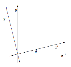
\[\begin{aligned} x^{\prime} &=+\cos (\theta) x+\sin (\theta) y \\ y^{\prime} &=-\sin (\theta) x+\cos (\theta) y \end{aligned}.\]
If f(x, y) is some function of location on the plane, then write expressions for
\[\frac{\partial f}{\partial x^{\prime}} )_{y^{\prime}}, \quad \frac{\partial f}{\partial y^{\prime}} )_{x^{\prime}}, \quad \text { and } \quad \frac{\partial f}{\partial x} )_{y^{\prime}}\]
in terms of
\[\frac{\partial f}{\partial x} )_{y} \quad \text { and } \quad \frac{\partial f}{\partial y} )_{x}.\]
Interpret ∂f/∂x)y' geometrically as a directional derivative. (That is, ∂f/∂x)y' is the slope of f along which curve in the plane?) Given this interpretation, does it have the expected limits as θ → 0 and as θ → π/2?
3.10 Maxwell relations for a three-variable system
Suppose Φ(x, y, z) satisfies
\[d \Phi=A(x, y, z) d x+B(x, y, z) d y+C(x, y, z) d z.\]
State three Maxwell relations relating various first derivatives of A(x, y, z), B(x, y, z), and C(x, y, z), and a fourth Maxwell relation relating various second derivatives of these functions.
3.11 The cylinder model with three variables
In the “three-variable cylinder model” the cylinders are described by height h, radius r, and density ρ. The master function is mass M(h, r, ρ), and the master equation is
\[d M(h, r, \rho)=\rho S(h, r) d r+\rho T(r) d h+V(h, r) d \rho ,\]
where S(h, r) is the side area, T(r) is the top area, and V(h, r) is the volume. Perform a Legendre transformation to a description in terms of the variables h, S, and ρ using the new master function
\[\Phi(h, S, \rho)=M-\rho S r.\]
a. Write down the new master equation.
b. Write down the three first-order Maxwell relations and confirm their correctness using explicit formulas such as M(h, S, ρ) = ρS2/(4πh).
c. Interpret Φ(h, S, ρ) physically.
3.12 Multivariate chain rule
Invent a problem going through the chain rule argument of section 3.8.1 with the cylinder model.
3.13 Contours of constant side area
Find contours of constant side area preparing for/using the technique of section 3.8.3.