17.3: The Gibbs Phase Rule

Up to this point the thermodynamical systems that we have been considering have consisted of just a single component and, for the most part, just one phase, but we are now going to discuss systems consisting of more than one phase and more than one component. The Gibbs Phase Law provides a relation between the number of phases, the number of components and the number of degrees of freedom. But Whoa, there! We have been using several technical terms here: Phase, Component, Degrees of Freedom. We need to describe what these mean.

The state of a system consisting of a single component in a single phase (for example a single gas – not a mixture of different gases) can be described by three intensive state variables, P, V and T. (Here V is the molar volume – i.e. the reciprocal of the density in moles per unit volume – and is an intensive variable.) That is, the state of the system is described by a point in three-dimensional PVT space. However, the intensive state variables are connected by an equation of state f(P, V, T) = 0, so that the system is constrained to be on the two-dimensional surface described by this equation. Thus, because of the constraint, only two intensive state variables suffice to describe the state of the system. Just two of the intensive state variables can be independently varied. The system has two degrees of freedom.

Definition. A phase is a chemically homogeneous volume, solid, liquid or gas, with a boundary separating it from other phases.

Definition. The number of intensive state variables that can be varied independently without changing the number of phases in a system is called the number of degrees of freedom of the system.

These are easy. Defining the number of components in a system needs a bit of care. I give a definition, but what the definition means can, I hope, be made a little clearer by giving a few examples.

Definition. The number of components in a system is the least number of constituents that are necessary to describe the composition of each phase.

Let us look at a few examples to try and grasp what this means.

First, let us consider an aqueous solution of the chlorides and bromides of sodium and potassium co-existing with the crystalline solids NaCl, KCl, NaBr, KBr, illustrated schematically in figure XVII.1.

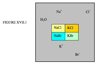
There are five phases – four solid and one liquid – but how many components? There are six elements: H, O, Na, K, Cl, B – but the quantities of each cannot be varied independently. There are two constraints: n(H) = 2n(O), and n(Na) + n(K) = n(Cl) + n(Br). That is, if we know the number of hydrogen atoms, then the number of oxygen atoms is known. And if we know the number of any three of Na, K, Cl or Br, then the fourth is known. Thus the number of constituents that that can be independently varied is four. The number of components is four.

Or again, consider an aqueous solution of a moles of H₂SO₄ in b moles of water. There is just one phase. There are three elements: H, O and S. These may be distributed among several species, such as H₂O, H₂SO₄, H₃O⁺, OH⁻, SO₄⁻⁻, but that doesn’t matter. There is just one constraint, namely that

2(a + b)n(H) = an(S) + (4a + b)n(O) .

That is, if we know the number of any two of H, O or S, we also know the number of the third. The number of components is two.

Or again, consider the reversible reaction

CaCO₃ (s) ↔ CaO (s) + CO₂ (g) .

If the system is in equilibrium, and we know the numbers of any two of these three molecules, the number of the third is determined by the equilibrium constant. Thus the number of components is two.

In each of these three examples, it was easy to state the number of phases and slightly more difficult to determine the number of components. We now need to ask ourselves what is the number of degrees of freedom. This is what the Gibbs phase law is going to tell us.

If there are C components in a system, the composition of a particular phase is fully described if we know the mole fraction of C − 1 of the components, since the sum of the mole fractions of all the components must be 1. This is so for each of the P phases, so that there are in all P(C − 1) mole fractions to be specified, as well as any two of the intensive state variables P, V and T. Thus there are P(C − 1) + 2 intensive state variables to be specified. (The mole fraction of each component is an intensive state variable.) But not all of these can be independently varied, because the molar Gibbs functions of each component are the same in all phases. (To understand this important statement, re-read this argument in Chapter 14 on the Clausius-Clapeyron equation.) For each of the C components there are P − 1 equations asserting the equality of the specific Gibbs functions in all the phases. Thus the number of intensive state variables that can be varied independently without changing the number of phases – i.e. the number of degrees of freedom, F − is P(C − 1) + 2 − C(P − 1), or

\[F = C − P + 2.\]

This is the Gibbs Phase Rule.

In our example of the sodium and potassium salts, in which there were C = 4 components distributed through P = 5 phases, there is just one degree of freedom. No more than one intensive state variable can be changed without changing the number of phases.

In our example of sulphuric acid, there was one phase and two components, and hence three degrees of freedom.

In the calcium carbonate system, there were three phases and two components, and hence just one degree of freedom.

If we have a pure gas, there is one phase and one component, and hence two degrees of freedom. (We can vary any two of P, V or T independently.)

If we have a liquid and its vapour in equilibrium, there are two phases and one component, and hence F = 1. We can vary P or T, but not both independently if the system is to remain in equilibrium. If we increase T, the pressure of the vapour that remains in equilibrium with its liquid increases. The system is constrained to lie on a line in PVT space.

If we have a liquid, solid and gas co-existing in equilibrium, there are three phases and one component and hence no degrees of freedom. The system exists at a single point in PVT space, namely the triple point.

I have often been struck by the similarity of the Gibbs phase rule to the topological relation between the number of faces F, edges E and vertices V of a solid polyhedron (with no topological holes through it). This relation is F = E − V + 2. E.g.

\[ \begin{array} ~ & E & V & F \\ \text{Tetrahedron:} & 6 & 4 & 4 \\ \text{Cube:} & 12 & 8 & 6 \\ \text{Octahedron:} & 12 & 6 & 8 \end{array}\]

As far as I know there is no conceivable connection between this and the Gibbs phase rule, and I don’t even find it useful as a mnemonic. I think we just have to put it down as one of life’s little curiosities.

Since writing this section, I have added some additional material on binary and ternary alloys, which provide additional examples of the Gibbs phase rule. I have added these at the end of the chapter, as sections 17.9 and 17.10.