
3.8: Thermodynamics Applied to Fluids
( \newcommand{\kernel}{\mathrm{null}\,}\)
In the rest of this chapter we apply the general results of section 3.6, “The Thermodynamic Dance”, to particular concrete situations. We begin with fluids, that is, systems whose thermodynamic states are adequately described by giving the variables temperature T, volume V, and particle number N. Furthermore, in this section we will not allow particles to enter or leave our system, so only two variables, T and V, are needed.
3.8.1 Heat capacities
Is there any relation between
Cp(T,p)=T∂S∂T)p,
the heat capacity at constant pressure, and
CV(T,V)=T∂S∂T)V,
the heat capacity at constant volume? Remembering that entirely different experiments are used to measure the two quantities, you might guess that there is not. But mathematically, the difference between Cp and CV is related to a change in variable from (T, V) to (T, p), so you might begin to suspect a relation. [You might want to prepare for this section by working problem 3.12.]
Begin with the mathematical definition of the total differential of entropy,
dS=∂S∂T)VdT+∂S∂V)TdV.
The above holds for any infinitesimal change. We restrict ourselves to infinitesimal changes at constant pressure, and divide by dT, to find
∂S∂T)p=∂S∂T)V+∂S∂V)T∂V∂T)p.
Multiplying both sides by T gives a heat capacity relation
Cp=CV+T∂S∂V)T∂V∂T)p.
This relationship is correct but not yet written in its most convenient form. For example, reference books provide tabulations of Cp and CV, but not of ∂S/∂V)T or ∂V/∂T)p.
The first step in changing the heat capacity relation into “standard form” is an easy one. Recall from problem 1.2 that the expansion coefficient (an intensive tabulated quantity6) is defined by
β(T,p)=1V∂V∂T)p
whence
Cp=CV+TVβ∂S∂V)T.
The second step is less obvious. At equation (3.71) I discussed the Maxwell relation
∂S∂V)T=∂p∂T)V,
and mentioned that the right hand side was much easier to measure. Thus we have the preferable expression
Cp=CV+TVβ∂p∂T)V.
This expression is still not very convenient, however, because the quantity ∂p/∂T)V is neither named nor tabulated. Although easier to measure than ∂S/∂V)T is, its measurement still requires a constant-volume strong box. Measurements at constant pressure are easier to perform and hence more frequently tabulated. We now write ∂p/∂T)V in terms of such quantities.
The total differential of V(T, p) is
dV=∂V∂T)pdT+∂V∂p)Tdp
or, in terms of named quantities,
dV=VβdT−VκTdp.
(The isothermal compressibility
κT(T,V)≡−1V∂V∂p)T
was defined in problem 1.2.) Restricting the above total differential to changes at constant V gives
VβdT=VκTdp
or
βκT=∂p∂T)V.
This immediately gives us the final form for our relationship between heat capacities,
Cp=CV+TVβ2κT.
This is a far from obvious result that is true for all fluids and, I emphasize, was derived assuming only that entropy exists and without the use of any explicit formula for the entropy.
Note that T, V, and κT are all positive quantities. The expansion coefficient β may be either positive or negative, but it enters the relationship as β2. Thus
Cp≥CV.
Can we understand these results physically? Heat capacity is the amount of heat required to raise the temperature of a sample by one kelvin. If the sample is heated at constant volume, all of the heat absorbed goes into increasing the temperature. But if the sample is heated at constant pressure, then generally the substance will expand as well as increase its temperature, so some of the heat absorbed goes into increasing the temperature and some is converted into expansion work. Thus we expect that more heat will be needed for a given change of temperature at constant pressure than at constant volume, i.e. that Cp ≥ CV. We also expect that the relation between Cp and CV will depend upon the expansion coefficient β. It is hard, however, to turn these qualitative observations into the precise formula (3.117) without recourse to the formal mathematics that we have used. It is surprising, for example, that β enters into the formula as β2, so that materials which contract with increasing temperature still have Cp ≥ CV.
For solids and liquids, there is little expansion and thus little expansion work, whence Cp ≈ CV. But for gases, Cp≫CV. What happens at two-phase coexistence?
So far we have discussed only the difference between the two heat capacities. It is conventional to also define the “heat capacity ratio”
γ≡CpCV,
which can be regarded as a function of T and V or as a function of T and p. But the result above shows that for all values of T and V,
γ(T,V)≥1.
We can apply these results to the ideal gas with equation of state
pV=NkBT.
Problem 1.2 used this equation to show that for an ideal gas,
β=1T and κT=1p.
Thus the heat capacity relation (3.117) becomes
Cp=CV+TVpT2=CV+pVT=CV+kBN,
and we have
γ=CpCV=1+kBNCV.
3.8.2 Energy as a function of temperature and volume
You know that E(S, V) is a master function with the famous master equation
dE=TdS−pdV.
For the variables T and V the master function is the Helmholtz potential F(T, V) with master equation
dF=−SdT−pdV.
Thus in terms of the variables T and V the energy in no longer a master function, but that doesn’t mean that it’s not a function at all. It is possible to consider the energy as a function of T and V, and in this subsection we will find the total differential of E(T, V). We begin by finding the total differential of S(E, V) and finish off by substituting that expression for dS into the master equation (3.125). The mathematical expression for that total differential is
dS=∂S∂T)VdT+∂S∂V)TdV,
but we showed in the previous subsection that this is more conveniently written as
dS=CVTdT+βκTdV.
Thus
dE=TdS−pdV=T[CVTdT+βκTdV]−pdV
and, finally,
dE=CVdT+[TβκT−p]dV.
The most interesting consequence of this exercise is that the heat capacity CV, which was defined in terms of an entropy derivative, is also equal to an energy derivative:
CV(T,V)≡T∂S∂T)V=∂E∂T)V.
For an ideal gas
[TβκT−p]=0,
whence
dE=CVdT+0dV.
Thus the energy, which for most fluids depends upon both temperature and volume, depends in the ideal gas only upon temperature:
E(T,V)=E(T).
and the heat capacity ratio
γ(T)=1+kBNCV(T).
Thermodynamics proves that for an ideal gas CV depends only upon T and not V, but experiment shows that in fact CV is almost independent of T as well. From the point of view of thermodynamics this is just an unexpected experimental result and nothing deeper. From the point of view of statistical mechanics this is not just a coincidence but is something that can be proved. . . we will do so in chapter 5.
3.8.3 Quasistatic adiabatic processes
This topic, titled by a string of polysyllabic words, sounds like an arcane and abstract one. In fact it has direct applications to the speed of sound, the manufacture of refrigerators, to the inflation of soccer balls, and to the temperature of mountain tops. [You might want to prepare for this section by working problem 3.13.]
If a fluid is changed in a quasistatic, adiabatic manner, its entropy will remain constant during the change. So, for example, if the state of the system is described by the two variables temperature and volume, then during a quasistatic adiabatic process the system will move along contour lines7 of constant entropy in the (T, V) plane, such as those below.
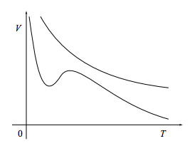
Our aim in this section is to find an equation V(T) for such constant-entropy contours.
We begin with the now-familiar total differential for the entropy as a function of temperature and volume,
dS=CVTdT+βκTdV.
This equation holds for any infinitesimal change, but we will apply it now to changes along an entropy contour, i.e. changes for which dS = 0. For such changes
βκTdV=−CVTdT
whence the differential equation for an entropy contour is
dV(T)dT=−CV(T,V)κT(T,V)Tβ(T,V).
The quantities on the right are usually (not always) positive, so the entropy contours usually (not always) slope downward. This is as much as we can say for a general fluid.
But for an ideal gas we can fill in the functions on the right to find
dV(T)dT=−CV(T)p(T,V)=−CV(T)VNkBT.
Using equation (3.136), this result is often written in the form
dV(T)dT=11−γ(T)VT.
This is as far as we can go for an arbitrary ideal gas.
But for an ideal gas with constant heat capacity, and hence with constant γ, this differential equation is readily solved using separation of variables. We write
(1−γ)dVV=dTT
with the immediate solution
(1−γ)lnV=lnT+ constant,
giving
V1−γ= constant T or TVγ−1= constant.
Remembering that γ ≥ 1, this confirms the downward slope of the entropy contours on the (V, T) plane. This result is most frequently used with the variables p and T, rather than V and T:
pVγ= constant .
The above equation holds only for quasistatic, adiabatic processes in ideal gases that have heat capacities independent of temperature. You might think that it is such a restricted result that it holds little interest. This equation is used frequently in applications, in the graduate record examination, and in physics oral examinations! You should memorize it and know how to work with it.
Problems
3.29 Intensive vs. extensive variables
Equation (3.134), E(T, V) = E(T), states that for an ideal gas the energy is a function of temperature alone. How is it possible for E, an extensive quantity, to be a function of only T, an intensive quantity?
3.30 Heat capacity at constant pressure
Equation (3.131) shows that the heat capacity at constant volume, which is defined in terms of an entropy derivative, is also equal to an energy derivative. You might suspect a similar relation between Cp(T, p, N) and
∂E(T,p,N)∂T)p,N.
Show that such a suspicion is not correct, and instead find an expression for Cp in terms of a derivative of enthalpy.
3.31 Qualitative heat capacity relations
(This problem is stolen from a GRE Physics test.)
For an ideal gas, Cp is greater than CV because:
a. The gas does work on its surroundings when its pressure remains constant while its temperature is increased.
b. The heat input per unit increase in temperature is the same for processes at constant pressure and at constant volume.
c. The pressure of the gas remains constant when its temperature remains constant.
d. The increase in the gas’s internal energy is greater when the pressure remains constant than when the volume remains constant.
e. The heat needed is greater when the volume remains constant than when the pressure remains constant.
3.32 Heat capacities in a magnetic system
For a magnetic system (see equation (3.100)), show that
CH=T∂S∂T)H,CM=T∂S∂T)M,β=∂M∂T)H, and χT=∂M∂H)T
are related through
CM=CH−Tβ2/χT
3.33 Isothermal compressibility
a. Show that the isothermal compressibility, defined in problem 1.2 as
κT=−1V∂V∂p)T,N
is also given by
κT=1ρ∂ρ∂p)T=1ρ2∂ρ∂μ)T=1ρ2∂2p∂μ2)T,
where ρ is the number density N/V. Clue:
∂ρ∂p)T=∂ρ∂μ)T∂μ∂p)T.
b. What does this result tell you about the relation between density and chemical potential?
c. In part (a.) we began with a description in terms of the three variables T, p, N and then reduced it to an intensive-only description, which requires just two variables, such as µ and T. Reverse this process to show that
κT=VN2∂N∂μ)T,V=−1N∂V∂μ)T,N.
3.34 Pressure differential
By regarding pressure as a function of temperature T and number density ρ, show that
dp=βκTdT+1ρκTdρ.
3.35 Isothermal vs. adiabatic compressibility
In class we derived a remarkable relation between the heat capacities Cp and CV. This problem uncovers a similar relation between the isothermal and adiabatic compressibilities,
κT=−1V∂V∂p)T and κS=−1V∂V∂p)S.
The adiabatic compressibility κS is the compressibility measured when the fluid is thermally insulated. (It is related to the speed of sound: see problem 3.44.)
a. Use
dS=∂S∂T)pdT+∂S∂p)Tdp
to show that
∂T∂p)S=βTCp/V.
Sketch an experiment to measure this quantity directly.
b. From the mathematical relation
dV=∂V∂p)Tdp+∂V∂T)pdT
derive the multivariate chain rule
∂V∂p)S=∂V∂p)T+∂V∂T)p∂T∂p)S,
whence
κS=κT−β2TCp/V.
c. Finally, show that
γ≡CpCV=κTκS.
3.36 Change of chemical potential with temperature
Prove that
∂μ∂T)p,N=−SN
and that
∂μ∂T)V,N=−∂S∂N)T,V=−SN+βρκT.
How's that for weird?
6It is easy to see why ∂V/∂T)p itself is not tabulated. Instead of requiring a tabulation for iron, you would need a tabulation for a five gram sample of iron, for a six gram sample of iron, for a seven gram sample of iron, etc.
7Such contours are sometimes called isoentropic curves or, even worse, adiabats. The latter name is not just a linguistic horror, it also omits the essential qualifier that only quasistatic adiabatic processes move along curves of constant entropy