9.5: Computer Simulation

9.5.1 Basic strategy

If we’re going to use a computer to solve problems in statistical mechanics, there are three basic strategies that we could take. I illustrate them here by showing how they would be applied to the Ising model.

1. Exhaustive enumeration. Just do it! List all the states (microstates, configurations), their associated probabilities, and average over them! Admittedly, there are a lot of states, but computers are fast, right? Let’s see how many states there are. Consider a pretty small problem: a three dimensional Ising model on an 8 × 8 × 8 cube. This system has 512 spins that can be oriented either “up” or “down”, so there are 2⁵¹² ≈ 10¹⁵⁴ configurations. Suppose that our computer could generate and examine a million configurations per second. . . this is about as fast as is currently possible. Then an exhaustive enumeration would require 10¹⁴⁸ seconds to do the job. By contrast, the universe is about 10¹⁸ seconds old. So for one computer to do the problem it would take 10¹³⁰ times the age of the universe. Now this is impractical, but maybe we could do it by arranging computers in parallel. Well, there are about 10⁸⁰ protons in the universe, and if every one were to turn into a spiffy Unix workstation, it would still require 10⁵⁰ times the age of the universe to complete the list. And this is for a small problem! Sorry, computers aren’t fast, and they never will be fast enough to solve the complete enumeration problem. It is not for nothing that this technique is called exhaustive enumeration.

2. Random sampling. Instead of trying to list the entire pool of possible configurations, we will dip into it at random and sample the configurations. This can be implemented by scanning through the lattice and orienting spins up with probability \(\frac{1}{2}\) and down with probability \(\frac{1}{2}\). The problem in this strategy is that all configurations are equally likely to be sampled, but because there are many more high energy configurations than low energy configurations, it is very unlikely to sample a low energy configuration (the “poker paradox” again). But in the Boltzmann distribution e^{−energy/k_BT} the low energy configurations are in fact more likely to occur. So you could sample for a long time before encountering even one configuration with non-negligible probability. This strategy is considerably better than the first one, but it would still take about the age of the universe to implement.

3. Importance sampling. This strategy is to sample the pool of possible configurations not completely at random, but in such a way that the most likely configurations are most likely to be sampled. An enormously successful algorithm to perform importance sampling was developed by Nick Metropolis and his coworkers Arianna Rosenbluth, Marshall Rosenbluth, Augusta Teller, and Edward Teller (of hydrogen bomb fame) in 1953. (“Equation of state calculations by fast computing machines”, J. Chem. Phys. 21 1087–1092.) It is called “the Metropolis algorithm”, or “the M(RT)² algorithm”, or simply “the Monte Carlo algorithm”. The next section treats this algorithm in detail.

An analogy to political polling is worth making here. Exhaustive enumeration corresponds to an election, random sampling corresponds to a random poll, and importance sampling corresponds to a poll which selects respondents according to the likelihood that they will vote.

9.5.2 The Metropolis algorithm

This algorithm builds a chain of configurations, each one modified (usually only slightly) from the one before. For example, if we number the configurations (say, for the 8 ×8×8 Ising model, from 1 to 2⁵¹²) such a chain of configurations might be

\[ C_{171} \rightarrow C_{49} \rightarrow C_{1294} \rightarrow C_{1294} \rightarrow C_{171} \rightarrow C_{190} \rightarrow \cdots\]

Note that it is possible for two successive configurations in the chain to be identical.

To build any such chain, we need some transition probability rule W(C_a → C_b) giving the probability that configuration C_b will follow configuration C_a. And to be useful for importance sampling, the rule will have to build the chain in such a way that the probability of C_n appearing in the chain is e^−βE_n/Z.

So we need to produce a result of the form: if “rule” then “Boltzmann probability distribution”. It is, however, very difficult to come up with such results. Instead we go the other way to produce a pool of plausible transition rules. . . plausible in that they are not obviously inconsistent with a Boltzmann probability distribution.

Consider a long chain of N_configs configurations, in which the probability of a configuration appearing is given by the Boltzmann distribution. The chain must be “at equilibrium” in that

\[ \text { number of transitions }\left(C_{a} \rightarrow C_{b}\right)=\text { number of transitions }\left(C_{b} \rightarrow C_{a}\right).\]

But the number of Cas in the chain is Nconfigse −βEa /Z, and similarly for the number of Cbs, so the equation above is

\[ N_{\text { configs }} \frac{e^{-\beta E_{a}}}{Z} W\left(C_{a} \rightarrow C_{b}\right)=N_{\text { configs }} \frac{e^{-\beta E_{b}}}{Z} W\left(C_{b} \rightarrow C_{a}\right),\]

whence

\[ \frac{W\left(C_{a} \rightarrow C_{b}\right)}{W\left(C_{b} \rightarrow C_{a}\right)}=e^{-\beta\left(E_{b}-E_{a}\right)}\]

This condition, called “detailed balance”, defines our pool of plausible transition probability rules. It is possible that a rule could satisfy detailed balance and still not sample according to the Boltzmann distribution, but any rule that does not satisfy detailed balance certainly cannot sample according to the Boltzmann distribution. In practice, all the rules that satisfy detailed balance seem to work.

Two transitions probability rules that do satisfy detailed balance, and the two rules most commonly used in practice, are

\[ W\left(C_{a} \rightarrow C_{b}\right)=[\text { normalization constant }]\left\{\frac{e^{-\beta \Delta E}}{1+e^{-\beta \Delta E}}\right\}\]

\[ W\left(C_{a} \rightarrow C_{b}\right)=[\text { normalization constant }]\left\{\begin{aligned} 1 & \text { if } \Delta E \leq 0 \\ e^{-\beta \Delta E} & \text { if } \Delta E>0 \end{aligned}\right\}\]

where we have taken

\[ \Delta E=E_{b}-E_{a}\]

and where the normalization constant is fixed so that

\[ \sum_{C_{b}} W\left(C_{a} \rightarrow C_{b}\right)=1.\]

If we had to calculate the normalization constant, then we would be back to performing an exhaustive enumeration, so we must find a way to work with unnormalized transition probabilities. To this end we define w_a→b as the factor for the transition probability aside from the normalization constant, i.e. the part in curly brackets in equations (9.61) and (9.62). Note that it is a positive number less than or equal to one:

\[ 0<\{\quad\} \equiv w_{a \rightarrow b} \leq 1.\]

Notice that for any rule satisfying detailed balance the transition probability must increase as the change in energy decreases, suggesting a simple physical interpretation: The chain of configurations is like a walker stepping from configuration to configuration on a “configuration landscape”. If a step would decrease the walker’s energy, he is likely to take it, whereas if it would increase his energy, he is likely to reject it. Thus the walker tends to go downhill on the configuration landscape, but it is not impossible for him to go uphill. This seems like a recipe for a constantly decreasing energy, but it is not, because more uphill steps than downhill steps are available to be taken.³

³This paragraph constitutes the most densely packed observation in this book. It looks backward to the poker paradox, to the definition of temperature, and to the “cash incentives” interpretation of the canonical ensemble. It looks forward to equilibration and to optimization by Monte Carlo simulated annealing. Why not read it again?

From these ingredients, Metropolis brews his algorithm:

Generate initial configuration [at random or otherwise]

Gather data concerning configuration [e.g. find M :=n_↑ − n_↓; M_sum:=M]

DO Iconfig = 2, Nconfigs

Generate candidate configuration [e.g. select a spin to flip]

Compute w_a→b for transition to candidate

With probability w_a→b, make the transition

Gather data concerning configuration [e.g. find M:=n_↑ − n_↓; M_sum:=M_sum + M]

END DO

Summarize and print data [e.g. M_ave:=M_sum/Nconfigs]

I’ll make three comments concerning this algorithm. First of all, note that the step “With probability w_a→b, make the transition” implies that sometimes the transition is not made, in which case two configurations adjacent in the chain will be identical. It is a common misconception that in this case the repeated configuration should be counted only once, but that’s not correct: you must execute the “Gather data concerning configuration” step whether the previous candidate was accepted or rejected.

Secondly, I wish to detail how the step

With probability w_a→b, make the transition

is implemented. It is done by expanding the step into the two substeps

Produce a random number z [0 ≤ z < 1]

IF z < w_a→b THEN switch to candidate

[i.e. configuration := candidate configuration]

Finally, I need to point out that this algorithm does not precisely implement either of the transition probability rules (9.61) or (9.62). For example, if the step “Generate candidate configuration” is done by selecting a single spin to flip, then the algorithm will never step from one configuration to a configuration three spin-flips away, regardless of the value of ∆E. Indeed, under such circumstances (and if there are N spins in the system), the transition probability rule is

\[ W\left(C_{a} \rightarrow C_{b}\right)=\left\{\begin{array}{cc}{\frac{1}{N} w_{a \rightarrow b}} & {\text { if } C_{a} \text { and } C_{b} \text { differ by a single spin flip }} \\ {0} & {\text { if } C_{a} \text { and } C_{b} \text { differ by more than a single spin flip }} \\ {1-\sum_{C_{b} \neq C_{a}} W\left(C_{a} \rightarrow C_{b}\right)} & {\text { if } C_{a}=C_{b}}\end{array}\right..\]

It is easy to see that this transition probability rule satisfies detailed balance.

9.5.3 Implementing the Metropolis algorithm

It is not atypical to run a Monte Carlo program for about 10,000 Monte Carlo steps per site. As such, the program might run for hours or even days. This is considerably less than the age of the universe, but probably far longer than you are used to running programs. The following tips are useful for speeding up or otherwise improving programs implementing the Metropolis algorithm.

1. Use scaled quantities. The parameters J, m, H, and T do not enter in any possible combination, but only through two independent products. These are usually taken to be

\[ \tilde{T}=\frac{k_{B} T}{J} \quad \text { and } \quad \tilde{H}=\frac{m H}{J}.\]

Thus the Boltzmann exponent for a given configuration is

\[ -\frac{E}{k_{B} T}=\frac{1}{\tilde{T}}\left(\sum_{\langle i, j\rangle} s_{i} s_{j}+\tilde{H} \sum_{i} s_{i}\right),\]

where s_i is +1 if the spin at site i is up, −1 if it is down, and where \(\langle i, j \rangle\) denotes a nearest neighbor pair.

2. Don’t find total energies. To calculate w_a→b you must first know ∆E, and the obvious way to find ∆E is to find E_b and E_a (through equation (9.68)) and subtract. This way is obvious but terribly inefficient. Because the change in configuration is small (usually a single spin flip) the change in energy can be found from purely local considerations without finding the total energy of the entire system being simulated. Similarly, if you are finding the average (scaled) magnetization

\[ M=n_{\uparrow}=n_{\downarrow}=\sum_{i} s_{i}\]

(as suggested by the square brackets in the algorithm on page 202) you don’t need to scan the entire lattice to find it. Instead, just realize that it changes by ±2 with each spin flip.

3. Precompute Boltzmann factors. It is computationally expensive to find evaluate a exponential, yet we must know the value of e^−β∆E. However, usually there are only a few possible values of ∆E. (For example in the square lattice Ising model with nearest neighbor interactions and a field, a single spin flip gives rise to one of only ten possible values of the energy change.) It saves considerable computational time (and often makes the program clearer) to precalculate the corresponding values of w_a→b just once at the beginning of the program, and to store those values in an array for ready reference when they are needed.

4. Average “on the fly”. The algorithm on page 202 finds the average (scaled) magnetization by summing the magnetization of each configuration in the chain and then dividing by the number of configurations. Because the chain is so long this raises the very real possibility of overflow in the value of M_sum. It is often better to keep a running tally of the average by tracking the “average so far” through

\[ M_{\mathrm{ave}} :=M_{\mathrm{ave}}(\text { Iconfig }-1) / \text { Iconf } \mathrm{ig}+M / \text { Iconfig }\]

or (identical mathematicall but preferable for numerical work)

\[ M_{\mathrm{ave}} :=M_{\mathrm{ave}}+\left(M-M_{\mathrm{ave}}\right) / \text { Iconfig. }.\]

5. Finite size effects. Use periodic or skew-periodic boundary conditions.

6. Lattice data structures. Suppose we wish to simulate a two-dimensional Ising model on a 4 × 3 square grid. An obvious data structure to hold the configuration in the computer’s memory is an integer-valued two-dimensional array declared through the code

INTEGER, PARAMETER :: Nx = 4, Ny = 3

INTEGER :: Spin (1:Nx, 1:Ny)

(I use the notation of Fortran 90. If you are familiar with some other computer language, the intent should nevertheless be clear.) If the spin at site (3,2) is up, then Spin(3,2) = +1, and if that spin is down, then Spin(3,2) = −1. The lattice sites are labeled as shown in this figure:

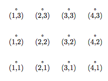
Although this representation is obvious, it suffers from a number of defects. First, it is difficult to generalize to other lattices, such as the triangular lattice in two dimensions or the face-centered cubic lattice in three dimensions. Second, finding the nearest neighbors of boundary sites using periodic or skew-periodic boundary conditions is complicated. And finally because the array is two-dimensional, any reference to an array element involves a multiplication,⁴ which slows down the finding of data considerably.

All of these defects are absent in the folded array representation of the lattice sites. In this representation the sites are stored as an integer-valued one-dimensional array declared through

INTEGER, PARAMETER :: Nx = 4, Ny = 3, NSites = Nx*Ny

INTEGER :: Spin (0:NSites-1)

Now the lattice sites are labeled as:

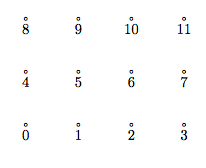
It is not hard to show that, with skew-periodic boundary conditions, the four neighbors of site number l (l for location) are

(l + 1) mod NSites, (l − 1) mod NSites, (l + Nx) mod NSites, (l − Nx) mod NSites.

Unfortunately, the Fortran Mod function was inanely chosen to differ from the mathematical mod function, so this arithmetic must be implemented through

Mod(l + 1, NSites)

Mod(l + (NSites - 1), NSites)

Mod(l + Nx, NSites)

Mod(l + (NSites - Nx), NSites)

7. Random number generators. It is hard to find an easy source of high-quality random numbers: this is a problem for physics, also for government and industry.

⁴In Fortran, the datum Site(i,j) is stored at memory location number i + j*(Nx-1), whence the data are stored in the sequence (1,1), (2,1), (3,1), (4,1), (1,2), (2,2),. . . . In other computer languages the formula for finding the memory location is different, but in all languages it involves an integer multiply

D.E. Knuth, Seminumerical Algorithms (Addison–Wesley, Reading, Massachusetts, 1981) chapter 3.

W.H. Press, S.A. Teukolsky, W.T. Vettering, and B.P. Flannery, Numerical Recipes chapter 7. (For a confession and a prize announcement, see also W.H. Press and S.A. Teukolsky, “Portable random number generators”, Computers in Physics 6 (1992) 522–524.)

T.-W. Chiu and T.-S. Guu, “A shift-register sequence random number generator,” Computer Physics Communications 47 (1987) 129–137. (See particularly figures 1 and 2.)

A.M. Ferrenberg, D.P. Landau, and Y.J. Wong, “Monte Carlo simulations: Hidden errors from ‘good’ random number generators,” Phys. Rev. Lett. 69 (1992) 3382.

S.K. Park and K.W. Miller, “Random number generators: Good ones are hard to find,” Communications of the ACM 31 (1988) 1192–1201.

8. Initial configurations and equilibration. The Metropolis algorithm does not specify how to come up with the first configuration in the chain. Indeed, selecting this configuration is something of an art. If you are simulating at high temperatures, it is usually appropriate to begin with a configuration chosen at random, so that about half the spins will be up and half down. But if you are simulating at low temperatures (or at high fields) it might be better to start at the configuration with all spins up. Other possibilities are also possible. But however you select the initial configuration, it is highly unlikely that the one you pick will be “typical” of the configurations for the temperature and magnetic field at which you are simulating.

9. Low temperatures. At low temperatures, most candidate transitions are rejected. BLK algorithm. (A.B. Bortz, J.L. Lebowitz, and M.H. Kalos, “A new algorithm for Monte Carlo simulation of Ising spin systems,” J. Comput. Phys. 17 (1975) 10–18.)

10. Critical temperatures. “Critical slowing down,” response is cluster flipping. (U. Wolff, “Collective Monte Carlo updating for spin systems,” Phys. Rev. Lett. 62 (1989) 361–364. See also Jian-Sheng Wang and R.H. Swendsen, “Cluster Monte Carlo algorithms,” Physica A 167 (1990) 565–579.)

11. First-order transitions.

12. Molecular dynamics.

9.5.4 The Wolff algorithm

In 1989 Ulli Wolff proposed an algorithm for Monte Carlo simulation that is particularly effective near critical points. (U. Wolff, Phys. Rev. Lett., 62 (1989) 361–364.) The next page presents the Wolff algorithm as applied to the zero-field ferromagnetic nearest-neighbor Ising model,

\[ \mathcal{H}=-J \sum s_{i} s_{j} \quad \text { with } \quad s_{i}=\pm 1,\]

on a square lattice or a simple cubic lattice.

Generate initial configuration

Gather data concerning this configuration

DO Iconfig = 2, Nconfigs

Select site j at random

Flip spin at j

Put j into cluster

NFlippedThisGeneration = 1

DO

IF (NFlippedThisGeneration = 0) EXIT

NFlippedPreviousGeneration = NFlippedThisGeneration

NFlippedThisGeneration = 0

FOR each previous generation member i of the cluster DO

FOR each neighbor j of i DO

IF (spin at j ≠ spin at i) THEN

with probability P = 1 − exp(−2J/k_BT)

Flip spin at j

Put j into cluster

NFlippedThisGeneration = NFlippedThisGeneration + 1

END IF

END DO

END DO

END DO

Gather data concerning this configuration

Empty the cluster

END DO

Summarize and print out results

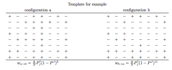
Demonstration of detailed balance. In these formulas,

\[ P_{J}=1-e^{-2 J / k_{B} T}.\]

The integer 8 is the number of sites in the cluster, 7 is the number of internal bonds in the skeleton, 5 is the number of external bonds leading to a + spin, and 11 is the number of external bonds leading to a − spin. The energy difference between configurations a and b depends only upon these last two integers. It is

\[ \Delta E=+2 J(5)-2 J(11)=-2 J(11-5).\]

Thus

\[ \frac{w_{a \rightarrow b}}{w_{b \rightarrow a}}=\left(1-P^{J}\right)^{5-11}=e^{-2 J(5-11) / k_{B} T}=e^{-\Delta E / k_{B} T}\]

and detailed balance is insured.