2.3: Barometric Formula and the Speed of Sound

Here we consider two simple examples of using the ideal gas law and the formula for adiabatic expansion.First, consider the barometric formula which gives the density (or pressure) of air at a height \(h\) above the surface of Earth (also called Pascal's principle). We assume complete equilibrium, mechanical, and thermal. The argument is illustrated in Figure \(\PageIndex{1}\).

Figure \(\PageIndex{1}\): Matching of forces for barometric formula

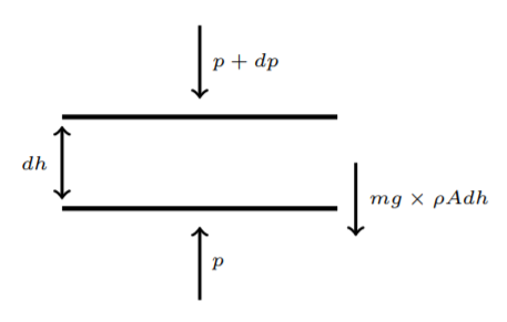
We consider a layer of air, with horizontal cross-sectional area \(A\) and height \(dh\). If we take the molecules to have a mass \(m\) and the number density of particles to be \(\rho\), then the weight of this layer of air is \(mg × \rho Adh\). This is the force acting downward. It is compensated by the difference of pressure between the upper boundary and the lower boundary for this layer. The latter is thus \(dp \times A\), again acting downward, as we have drawn it. The total force being zero for equilibrium, we get

\[dp\;A + mg\rho Adh = 0\]

Thus the variation of pressure with height is given by

\[\frac{dp}{dh} = −mg \rho\]

Let us assume the ideal gas law for air; this is not perfect, but is a reasonably good approximation. Then \(p = \frac{NkT}{V} = ρkT\) and the equation above becomes

\[\frac{dp}{dh} = −\frac{mg}{kT}p\]

The solution is

\[p = p_0 \exp \left(−\dfrac{mgh}{kT} \right),\]

or

\[ρ = ρ_0 \exp \left(−\dfrac{mgh}{kT} \right) \label{2.3.4} \]

This argument is admittedly crude. In reality, the temperature also varies with height. Further, there are so many nonequilibrium processes (such as wind, heating due to absorption of solar radiation, variation of temperature between day and night, etc.) in the atmosphere that Equation \ref{2.3.4} can only be valid for a short range of height and over a small area of local equilibrium.

Our next example is about the speed of sound. For this, we can treat the medium, say, air, as a fluid, characterized by a number density \(ρ\) and a flow velocity \(\vec{v}\). The equations for the fluid are

\[\begin{align} \frac{∂ρ}{∂t} + ∇ · (ρ \vec{v}) &= 0 \label{eq:A}\\[4pt] \frac{∂\vec{v}}{∂t} + v_i∂_i\vec{v} &= −\frac{∇p}{ρ} \label{eq:B}\end{align}\]

Equation \ref{eq:A} is the equation of continuity which expresses the conservation of particle number, or mass, if we multiply the equation by the mass of a molecule. Equation \ref{eq:B} is the fluid equivalent of Newton’s second law. In the absence of external forces, we still can have force terms; in fact the gradient of the pressure, as seen from the equation, acts as a force term. This may also be re-expressed in terms of the density, since pressure and density are related by the equation of state.

Now consider the medium in equilibrium with no sound waves in it. The equilibrium pressure should be uniform; we denote this by \(p_0\), with the corresponding uniform density as \(ρ_0\). Further, we have \(\vec{v} = 0\) in equilibrium. Now we can consider sound waves as perturbations on this background, writing

\[\begin{align*} ρ &= ρ_0 + δρ \\[4pt] p &= p_0 + δρ \left(\frac{∂p}{∂ρ}\right)_0 \\[4pt] \vec{v} &= 0 + \vec{v} \end{align*}\]

Treating \(δρ\) and \(\vec{v}\) as being of the first order in the perturbation, the fluid equations can be approximated as

\[\begin{align*} \frac{∂}{∂t}(δρ) &≈ −ρ_0 ∇ · \vec{v} \\[4pt] \frac{∂\vec{v}}{∂t} &≈ − \frac{1}{ρ_0} \left(\frac{∂p}{∂ρ}\right)_0 ∇δρ \end{align*}\]

Taking the derivative of the first equation and using the second, we find

\[\left(\frac{∂^2}{∂t^2} − c_s^2 ∇^2\right) δρ = 0 \label{2.3.8}\]

where

\[c_s^2= \left(\frac{∂p}{∂ρ}\right)_0\]

Equation \ref{2.3.8} is the wave equation with the speed of propagation given by \(c_s\). This equation shows that density perturbations can travel as waves; these are the sound waves. It is easy to check that the wave equation has wave-like solutions of the form

\[δρ = A\cos(ωt − \vec{k} · \vec{x}) + B\sin(ωt − \vec{k} · \vec{x})\]

with \(ω^2 = c_s^2 \vec{k} · \vec{k}\). This again identifies \(c_s\) as the speed of propagation of the wave.

We can calculate the speed of sound waves more explicitly using the equation of state. If we take air to obey the ideal gas law, we have \(p = ρ kT\). If the process of compression and de-compression which constitutes the sound wave is isothermal, then

\[\left(\frac{∂p}{∂ρ}\right)_0 = \frac{p_0}{ρ_0}.\]

Actually, the time-scale for the compression and de-compression in a sound wave is usually very short compared to the time needed for proper thermalization, so that it is more accurate to treat it as an adiabatic process. In this case, we have

\[pV^{\gamma} = \text{constant}\]

so that

\[c_s^2= \left(\frac{∂p}{∂ρ}\right)_0 = \gamma\frac{p_0}{ρ_0}\]

Since \(\gamma > 1\), this gives a speed higher than what would be obtained in an isothermal process. Experimentally, one can show that this formula for the speed of sound is what is obtained, showing that sound waves result from an adiabatic process.