
3.5: Some Other Thermodynamic Engines


- Last updated
- Mar 15, 2021
- Save as PDF

( \newcommand{\kernel}{\mathrm{null}\,}\)
We will now consider some other thermodynamic engines which are commonly used.
Otto Cycle
The automobile engine operates in four steps, with the injection of the fuel-air mixture into the cylinder. It undergoes compression which can be idealized as being adiabatic. The ignition then raises the pressure to a high value with almost no change of volume. The high pressure mixture rapidly expands, which is again almost adiabatic. This is the power stroke driving the piston down. The final step is the exhaust when the spent fuel is removed from the cylinder. This step happens without much change of volume. This process is shown in Fig. 3.4.2. We will calculate the efficiency of the engine, taking the working material to be an ideal gas.
Heat is taken in during the ignition cycle B to C. The heat comes from the chemical process of burning but we can regard it as heat taken in from a reservoir. Since this is at constant volume, we have
QH=Cv(TC−TB)
Heat is given out during the exhaust process D to A, again at constant volume, so
QL=Cv(TD−TA)
Further, states C and D are connected by an adiabatic process, so are A and B. Thus pVγ=nRTVγ−1 is preserved for these processes. Also, VA=VD, VB=VC, so we have
TD=TC(VBVA)γ−1,TA=TB(VBVA)γ−1
This gives
QL=Cv(TC−TB)(VBVA)γ−1
The efficiency is then
η=1−QLQH=1−(VBVA)γ−1
Diesel Cycle
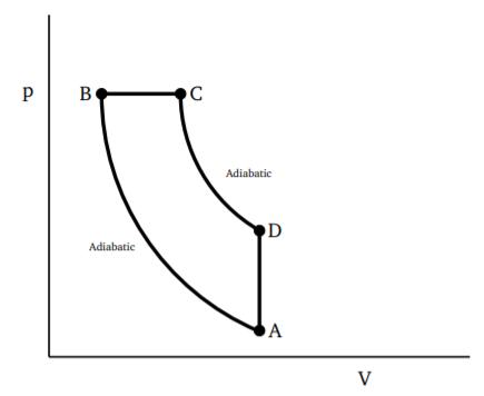
The idealized operation of a diesel engine is shown in Fig. 3.5.1. Initially, only air is admitted into the cylinder. It is then compressed adiabatically to very high pressure (and hence very high temperature). Fuel is then injected into the cylinder. The temperature in the cylinder is high enough to ignite the fuel. The injection of the fuel is controlled so that the burning happens at essentially constant pressure (B to C in figure). This is the key difference with the automobile engine. At the end of the burning process, the expansion continues adiabatically (part C to D). From D back to A we have the exhaust cycle as in the automobile engine.
Taking the air (and fuel) to be an ideal gas, we can calculate the efficiency of the diesel engine. Heat intake (from burning fuel) is at constant pressure, so that
QH=Cp(TC−TB)
Heat is given out (D to A) at constant volume so that
QL=Cp(TD−TA)
We also have the relations,
TA=TB(VBVA)γ−1,TD=TC(VCVA)γ−1
Further, pB=pC implies TB=TC(VBVC), which, in turn, gives
TA=TC(VBVC)(VBVA)γ−1
We can now write
QL=CvTC[(VCVA)γ−1−(TBVC)(VBVA)γ−1]=CvTC(VCVA)γ−1[1−(VBVC)γ]
QH=CpTC[1−VBVC]
These two equations give the efficiency of the diesel cycle as
η=1−1γ(VCVA)γ−1[1−(VBVC)γ1−(VBVC)]=1−1γ(TDTC)[1−(VBVC)γ1−(VBVC)]