8.2: Bose-Einstein Distribution

We will now consider the derivation of the distribution function for free bosons carrying out the counting of states along the lines of what we did for the Maxwell-Boltzmann distribution. Let us start by considering how we obtained the binomial distribution. We considered a number of particles and how they can be distributed among, say, \(K\) boxes. As the simplest case of this, consider two particles and two boxes. The ways in which we can distribute them are as shown below. The boxes may correspond to different values of momenta, say \(\vec{p_1}\) and \(\vec{p_2}\), which have

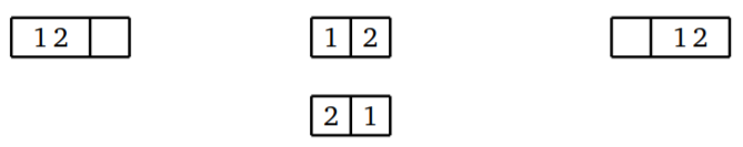
the same energy. There is one way to get the first or last arrangement, with both particles in one box; this corresponds to

\[W(2, 0) = \dfrac{2!}{2!0!}= \dfrac{2!}{0!2!} = W(0,2) \label{8.1}\]

There are two ways to get the arrangement of one particle in each box, corresponding to

\[W(1, 1) = \dfrac{2!}{1!1!} \label{8.2}\]

The generalization of this counting is what led us to the Maxwell-Boltzmann statistics. But if particles are identical with no intrinsic attributes distinguishing the particles we have labeled 1 and 2, this result is incorrect. The possible arrangements are just

Counting the arrangement of one particle per box twice is incorrect; the correct counting should give \(W(2, 0) = W(0, 2) = 1\) and \(W(1, 1) = 1\), giving a total of 3 distinct arrangements or states. To generalize this, we first consider \(n\) particles to be distributed in 2 boxes. The possible arrangements are \(n\) in box 1, 0 in box 2; \(n − 1\) in box 1, 1 in box 2; · · · ; 0 in box 1, \(n\) in box 2, giving \(n + 1\) distinct arrangements or states in all. If we have n particles and 3 boxes, we can take \(n − k\) particles in the first two boxes (with \(n − k + 1\) possible states) and k particles in the third box. But \(k\) can be anything from zero to \(n\), so that the total number of states is

\[\sum_{k=0}^{n}(n-k+1)=\frac{(n+2)(n+1)}{2}=\frac{(n+3-1) !}{n !(3-1) !}\]

We may arrive at this in another way as well. Represent the particles as dots and use 3 − 1 = 2 partitions to separate them into three groups. Any arrangement then looks like

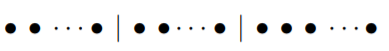
Clearly any permutation of the \(n + 2\) entities (dots or partitions) gives an acceptable arrangement. There are \((n + 2)!\) such permutations. However, the permutations of the two partitions do not change the arrangement, neither do the permutations of the dots among themselves. Thus, the number of distinct arrangements or states is

\[\frac{(n+2)!}{n!2!} = \frac{(n+2)(n+1)}{2} \]

Generalizing this argument, for \(g\) boxes and \(n\) particles, the number of distinct arrangements is given by

\[W = \frac{(n+g-1)!}{n!(g-1)!} \]

We now consider \(N\) particles, with \(n_1\) of them having energy \(\epsilon_1\) each, \(n_2\) of them with energy \(\epsilon_2\) each, etc. Further, let \(g_1\) be the number of states with energy \(\epsilon_1\), \(g_2\) the number of states with energy \(\epsilon_2\), etc. The degeneracy \(g_α\) may be due to different values of momentum (e.g., different directions of \(\vec{p}\) with the same energy \(\epsilon = \frac{p^2}{2m})\) or other quantum numbers, such as spin. The total number of distinct arrangements for this configuration is

\[W(\{n_{\alpha}\}) = \prod_{\alpha} \frac{(n_α+g_α-1)}{n_α!(g_α -1)!} \]

The corresponding entropy is \(k\; \log W\) and we must maximize this subject to \(\sum_α n_α = N\) and \(\sum_α n_α \epsilon_α = U\). With the Stirling formula for the factorials, the function to be extremized is thus

\[\frac{S}{k} − βU + βµN = \sum_α \left[ (n_α + g_α - 1) \log(n_α + g_α - 1) - (n_α + g_α - 1) - n_α \log n_α + n_α - \beta \epsilon_α n_α + \beta \mu n_α \right] + \text{terms independent of } n_α\]

The extremization condition is

\[\log \left[ \frac{n_α + g_α - 1}{n_α} \right] \]

with the solution

\[n_α = \frac{g_α}{e^{\beta(\epsilon_α - \mu)} - 1} \]

where we have approximated \(g_α − 1 ≈ g_α\), since the use of the Stirling formula needs large numbers. As the occupation number per state, we can take the result as

\[n = \frac{1}{e^{\beta(\epsilon_α - \mu)} - 1} \label{8.1.10}\]

with the degeneracy factors arising from the summation over states of the same energy. This is the Bose-Einstein distribution. For a free particle, the number of states in terms of the momenta can be taken as the single-particle \(d\mathcal{N}\), which, from Equation 7.4.1, is

\[d\mathcal{N} = \frac{d^3xd^3p}{(2 \pi ħ)^3} \]

Thus the normalization conditions on the Bose-Einstein distribution are

\[\sum \int \frac{d^3xd^3p}{(2 \pi ħ)^3} \frac{1}{e^{\beta(\epsilon_α - \mu)} - 1} = N \\[4pt] \sum \int \frac{d^3xd^3p}{(2 \pi ħ)^3} \frac{ \epsilon }{e^{\beta(\epsilon_α - \mu)} - 1} = U \]

The remaining sum in this formula is over the internal states of the particle, such as spin states. It is also useful to write down the partition function \(Z\). Notice that we may write the occupation number \(n\) in Equation \ref{8.1.10} as

\[n = \frac{1}{\beta} \frac{\partial}{\partial \mu} \left[ -\log \left( 1 - e^{-\beta(\epsilon_α - \mu)} \right) \right] \]

This result holds for each state for which we are calculating \(n\). But recall that the total number \(N\) should be given by

\[N = \frac{1}{\beta} \frac{\partial}{\partial \mu} \log Z\]

Therefore, we expect the partition function to be given by

\[ \begin{equation}
\begin{split}
\log Z & = -\sum \log \left( 1 - e^{-\beta(\epsilon_α - \mu)} \right) \\[0.125in]
Z & = \prod \frac{1}{1 - e^{-\beta(\epsilon_α - \mu)}}
\end{split}
\end{equation} \]

For each state with fixed quantum numbers, we can write

\[ \begin{equation}
\begin{split}
\frac{1}{1 - e^{-\beta(\epsilon_α - \mu)}} & = 1 + e^{-\beta (\epsilon - \mu)} + e^{-2 \beta (\epsilon - \mu)} + e^{-3 \beta (\epsilon - \mu) } \\[0.125in]
& = \sum_n e^{-n \beta (\epsilon - \mu)}
\end{split}
\end{equation} \]

This shows that the partition function is the sum over states of possible occupation numbers of the Boltzmann factor \( e^{-beta (\epsilon - \mu)} \). This is obtained in a clearer way in the full quantum theory where

\[Z = \text{Tr}(e^{- \beta (\hat{H}- \mu \hat{N})}) \]

where \(\hat{H}\) and \(\hat{N}\) are the Hamiltonian operator and the number operator, respectively, and \(\text{Tr}\) denotes the trace over a complete set of states of the system.