8.10: Heat Capacities of Solids
( \newcommand{\kernel}{\mathrm{null}\,}\)
I do not deal a great deal with solid state physics in these notes, particularly in this chapter, which has been concerned mostly with gases. But the inclusion of the heat capacities of three metals in the above table provides an opportunity for a brief mention of the heat capacities of metals and of other crystalline solids. In a simple model of a crystalline solid, the solid can be thought of as a regular lattice of atoms held in position near their neighbors by springs, and the atoms have three degrees of vibrational freedom – in the x, y and z directions. For each of these vibrational modes there are two squared terms (of the form 12mv2 and 12Iω2 ) that contribute to the internal energy. The internal energy associated with each of these six terms is 12RT per mole, which comes to 3RT per mole, and thus you would expect the molar heat capacity to be about 3R – and you can see from the above table that this is indeed the case. Indeed at room temperature, most metals and simple crystalline solids have a molar heat capacity of about 3R. (This is sometimes referred to as “Dulong and Petit’s Rule”.) At low temperatures, however, the molar heat falls below this value, and eventually approaches zero at 0 K. At very low temperatures, the molar heat capacity varies roughly as the cube of the temperature. As room temperatures are reached, the molar heat capacity asymptotically approaches the “classical” value of 3R.
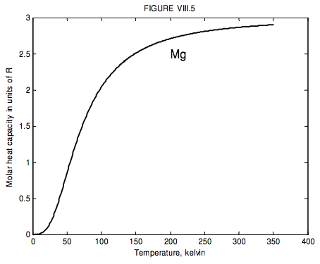
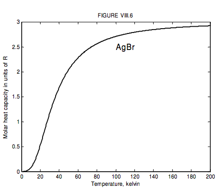
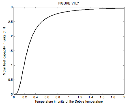
The run of molar heat capacity with temperature at low temperatures looks a little like figure VIII.5 for magnesium and figure VIII.6 for silver bromide. It will be seen that these two curves are the same shape except for a different scale along the temperature axis – and the same is true for most metals and simple crystalline solids. Indeed we can assign to each solid a characteristic temperature, known as the Debye temperature, θD, and then, if we express temperature not in kelvin but in units of the Debye temperature for the particular solid, then the curves are indeed the same shape. In other words, the molar heat capacity of all solids (or at least all solids that behave like this!) is the same function of T/θD. I show this function as figure VIII.7.
The theory of the heat capacities of solids was investigated by Einstein and by Debye. (Peter Debye – Dutch-American physicist/chemist. Nobel Chemistry prize 1936.) The Debye temperature is related to the vibrational frequency of the atoms in their crystalline lattice. Diamond is a very hard substance, with very strong interatomic bonds. Consequently the vibrational frequencies are very high, and the Debye temperature for diamond is correspondingly high: θD = 1860 K. As a result of this the heat capacity rises very slowly with increasing temperature, and at room temperature is well below the “classical” value of 3R. Most other solids have weaker bonds and far lower Debye temperatures, and consequently their molar heat capacities have almost reached the classical Dulong-Petit value of 3R at room temperature. Here are a few Debye temperatures:
| Elements | Debye temperature |
|---|---|
| Potassium | 100K |
| Silver bromide | 145 |
| Silver | 215 |
| Magnesium | 290 |
| Copper | 315 |
| Iron | 420 |
If it seems that the harder the solid the higher the Debye temperature and the slower the solid is to reach its classical CV of 3R, this is not coincidence.
I do not derive Debye’s theoretical formula here – it is something to look forward to in courses on solid state physics or statistical mechanics, but, for interest, the formula (which I used for calculating figures VIII.5-7) is
CV=9T3∫1/T0x4ex(ex−1)2dx.
In this equation CV is in units of R, and T is in units of the Debye temperature.


In case you are wondering what the symbol “x” stands for in equation 8.9.1, it is merely a dummy variable, for the integral in that expression is a function not of x but of T, the upper limit of the integral.
If you try to reproduce figure VIII.7 yourself by evaluating equation 8.9.1 for a number of different temperatures, you will soon find that it is a good deal more laborious than may at first be evident.
In my first attempt at doing it, for each of the 400 values of T that I used for plotting Figure VIII.7, I used a 1000 point Simpson’s Rule integration. Thus I evaluated the integrand 400,000 times, and it took the computer almost half a second. Later, I found that Gaussian quadrature was much, much more efficient, requiring the calculation of the integrand at only a very few points.
However, J. Viswanathan of Chennai, India, has since shown me an even better method than the Gaussian quadrature.
He uses the theorem
ddx∫g(x)0f(y)dy=f(g(x))g′(x)
This was a new one on me, but it is very easy to derive and looks almost obvious in hindsight. Applied to our problem, that is, applied to our equation
CV=9T3∫1/T0x4ex(ex−1)2dx,
it becomes, after a modest amount of work:
dCVdT=3CVT−9Tf(1/T),
where
f(x)=x4ex(ex−1)2.
He evaluates CV at T = 2, using a direct numerical integration of equation 8.9.1 - but this is the only time that he does this! The answer is 2.9628. Then he moves down by dT at each step and calculates the corresponding dCV by using a fourth order Runge-Kutta integration on the differential equation 8.9.3. The three methods agree very well, but the Simpson’s Rule method was by far the most laborious.
Debye’s theory was published in 1912, and they certainly didn’t have electronic computers, or even electronic hand calculators, in those days. In the 1950s most scientists were using hand-operated mechanical calculators, with electrically-driven mechanical calculators beginning to come into use towards the end of that decade. I suspect that in 1912 not even hand-operated mechanical calculators were available, and calculations would have been done using pencil and paper and logarithm and other tables. One must think of the physical insight and mathematical competence needed to develop the theory of the heat capacity in the first place, and then the enormous effort needed to calculate the resulting equations.


