Physics LibreTexts

11.2: The Carnot Cycle

  • Page ID
    7278
  • \( \newcommand{\vecs}[1]{\overset { \scriptstyle \rightharpoonup} {\mathbf{#1}} } \)

    \( \newcommand{\vecd}[1]{\overset{-\!-\!\rightharpoonup}{\vphantom{a}\smash {#1}}} \)

    \( \newcommand{\id}{\mathrm{id}}\) \( \newcommand{\Span}{\mathrm{span}}\)

    ( \newcommand{\kernel}{\mathrm{null}\,}\) \( \newcommand{\range}{\mathrm{range}\,}\)

    \( \newcommand{\RealPart}{\mathrm{Re}}\) \( \newcommand{\ImaginaryPart}{\mathrm{Im}}\)

    \( \newcommand{\Argument}{\mathrm{Arg}}\) \( \newcommand{\norm}[1]{\| #1 \|}\)

    \( \newcommand{\inner}[2]{\langle #1, #2 \rangle}\)

    \( \newcommand{\Span}{\mathrm{span}}\)

    \( \newcommand{\id}{\mathrm{id}}\)

    \( \newcommand{\Span}{\mathrm{span}}\)

    \( \newcommand{\kernel}{\mathrm{null}\,}\)

    \( \newcommand{\range}{\mathrm{range}\,}\)

    \( \newcommand{\RealPart}{\mathrm{Re}}\)

    \( \newcommand{\ImaginaryPart}{\mathrm{Im}}\)

    \( \newcommand{\Argument}{\mathrm{Arg}}\)

    \( \newcommand{\norm}[1]{\| #1 \|}\)

    \( \newcommand{\inner}[2]{\langle #1, #2 \rangle}\)

    \( \newcommand{\Span}{\mathrm{span}}\) \( \newcommand{\AA}{\unicode[.8,0]{x212B}}\)

    \( \newcommand{\vectorA}[1]{\vec{#1}}      % arrow\)

    \( \newcommand{\vectorAt}[1]{\vec{\text{#1}}}      % arrow\)

    \( \newcommand{\vectorB}[1]{\overset { \scriptstyle \rightharpoonup} {\mathbf{#1}} } \)

    \( \newcommand{\vectorC}[1]{\textbf{#1}} \)

    \( \newcommand{\vectorD}[1]{\overrightarrow{#1}} \)

    \( \newcommand{\vectorDt}[1]{\overrightarrow{\text{#1}}} \)

    \( \newcommand{\vectE}[1]{\overset{-\!-\!\rightharpoonup}{\vphantom{a}\smash{\mathbf {#1}}}} \)

    \( \newcommand{\vecs}[1]{\overset { \scriptstyle \rightharpoonup} {\mathbf{#1}} } \)

    \( \newcommand{\vecd}[1]{\overset{-\!-\!\rightharpoonup}{\vphantom{a}\smash {#1}}} \)

    \(\newcommand{\avec}{\mathbf a}\) \(\newcommand{\bvec}{\mathbf b}\) \(\newcommand{\cvec}{\mathbf c}\) \(\newcommand{\dvec}{\mathbf d}\) \(\newcommand{\dtil}{\widetilde{\mathbf d}}\) \(\newcommand{\evec}{\mathbf e}\) \(\newcommand{\fvec}{\mathbf f}\) \(\newcommand{\nvec}{\mathbf n}\) \(\newcommand{\pvec}{\mathbf p}\) \(\newcommand{\qvec}{\mathbf q}\) \(\newcommand{\svec}{\mathbf s}\) \(\newcommand{\tvec}{\mathbf t}\) \(\newcommand{\uvec}{\mathbf u}\) \(\newcommand{\vvec}{\mathbf v}\) \(\newcommand{\wvec}{\mathbf w}\) \(\newcommand{\xvec}{\mathbf x}\) \(\newcommand{\yvec}{\mathbf y}\) \(\newcommand{\zvec}{\mathbf z}\) \(\newcommand{\rvec}{\mathbf r}\) \(\newcommand{\mvec}{\mathbf m}\) \(\newcommand{\zerovec}{\mathbf 0}\) \(\newcommand{\onevec}{\mathbf 1}\) \(\newcommand{\real}{\mathbb R}\) \(\newcommand{\twovec}[2]{\left[\begin{array}{r}#1 \\ #2 \end{array}\right]}\) \(\newcommand{\ctwovec}[2]{\left[\begin{array}{c}#1 \\ #2 \end{array}\right]}\) \(\newcommand{\threevec}[3]{\left[\begin{array}{r}#1 \\ #2 \\ #3 \end{array}\right]}\) \(\newcommand{\cthreevec}[3]{\left[\begin{array}{c}#1 \\ #2 \\ #3 \end{array}\right]}\) \(\newcommand{\fourvec}[4]{\left[\begin{array}{r}#1 \\ #2 \\ #3 \\ #4 \end{array}\right]}\) \(\newcommand{\cfourvec}[4]{\left[\begin{array}{c}#1 \\ #2 \\ #3 \\ #4 \end{array}\right]}\) \(\newcommand{\fivevec}[5]{\left[\begin{array}{r}#1 \\ #2 \\ #3 \\ #4 \\ #5 \\ \end{array}\right]}\) \(\newcommand{\cfivevec}[5]{\left[\begin{array}{c}#1 \\ #2 \\ #3 \\ #4 \\ #5 \\ \end{array}\right]}\) \(\newcommand{\mattwo}[4]{\left[\begin{array}{rr}#1 \amp #2 \\ #3 \amp #4 \\ \end{array}\right]}\) \(\newcommand{\laspan}[1]{\text{Span}\{#1\}}\) \(\newcommand{\bcal}{\cal B}\) \(\newcommand{\ccal}{\cal C}\) \(\newcommand{\scal}{\cal S}\) \(\newcommand{\wcal}{\cal W}\) \(\newcommand{\ecal}{\cal E}\) \(\newcommand{\coords}[2]{\left\{#1\right\}_{#2}}\) \(\newcommand{\gray}[1]{\color{gray}{#1}}\) \(\newcommand{\lgray}[1]{\color{lightgray}{#1}}\) \(\newcommand{\rank}{\operatorname{rank}}\) \(\newcommand{\row}{\text{Row}}\) \(\newcommand{\col}{\text{Col}}\) \(\renewcommand{\row}{\text{Row}}\) \(\newcommand{\nul}{\text{Nul}}\) \(\newcommand{\var}{\text{Var}}\) \(\newcommand{\corr}{\text{corr}}\) \(\newcommand{\len}[1]{\left|#1\right|}\) \(\newcommand{\bbar}{\overline{\bvec}}\) \(\newcommand{\bhat}{\widehat{\bvec}}\) \(\newcommand{\bperp}{\bvec^\perp}\) \(\newcommand{\xhat}{\widehat{\xvec}}\) \(\newcommand{\vhat}{\widehat{\vvec}}\) \(\newcommand{\uhat}{\widehat{\uvec}}\) \(\newcommand{\what}{\widehat{\wvec}}\) \(\newcommand{\Sighat}{\widehat{\Sigma}}\) \(\newcommand{\lt}{<}\) \(\newcommand{\gt}{>}\) \(\newcommand{\amp}{&}\) \(\definecolor{fillinmathshade}{gray}{0.9}\)

    I referred above to one of the uses of the theoretical concept known as the Carnot cycle, namely that it enables us to define an absolute temperature scale. I suggest that, before you read any further, you re-read Section 3.4 of Chapter 3.

    Pause while you re-read Section 3.4

    As a temporary measure I am going to use the symbol θ to represent the temperature measured on the ideal gas scale. I shall then define an absolute temperature scale, T, and show that it is identical with the ideal gas temperature scale.

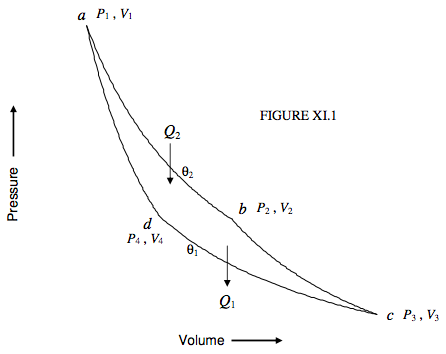
    To start with, I shall suppose that the working substance in our Carnot engine is an ideal gas. We shall refer to figure XI.1, in which ab and cd are isotherms at temperatures θ2 and θ1 respectively (θ2 > θ1), and bc and da are adiabats. Starting at the point a(P1, V1), a quantity of heat Q2 is supplied to the gas as it expands isothermally from a to b(P2 ,V2) at temperature θ2 on the ideal gas scale. During this phase, the cylinder is supposed to be uninsulated and placed in a hot bath at temperature θ2. As it expands isothermally it does external work. Since the working substance is an ideal gas, the internal energy at constant temperature is independent of volume (there is no internal work against van der Waals forces to be done) so the heat supplied to the gas is equal to the external work that it does. That is, per mole,

    \[ Q_{2}=R \theta_{2} \ln \left(V_{2} / V_{1}\right).\]

    Screen Shot 2019-07-04 at 6.46.07 PM.png

    After the gas has reached b the cylinder is insulated and the gas expands adiabatically and reversibly to c(P3, V3).

    It is then placed in a cold bath at temperature θ1, uninsulated, and compressed isothermally to d(P4, V4). During this stage it gives out a quantity of heat Q1:

    \[ Q_{1}=R \theta_{1} \ln \left(V_{3} / V_{4}\right).\]

    Finally it is insulated again and compressed adiabatically and reversibly to its original state a.

    For these four stages we have the equations

    \[ {l}{P_{1} V_{1}=P_{2} V_{2}}\]

    \[ {P_{2} V_{2}^{\gamma}=P_{3} V_{3}^{\gamma}}\]

    \[{P_{3} V_{3}=P_{4} V_{4}}\]

    \[{P_{1} V_{1}^{\gamma}=P_{4} V_{4}^{\gamma}}\]

    From these, we readily see that

    \[ V_{2} / V_{1}=V_{3} / V_{4},\]

    and therefore

    \[ Q_{2} / Q_{1}=\theta_{2} / \theta_{1}.\]

    The net heat received is Q2Q1, and this is the heat available for doing external work. A quantity of heat must be supplied at the beginning of each cycle, and so the efficiency of the cycle is

    \[ \eta=\frac{Q_{2}-Q_{1}}{Q_{2}}=\frac{\theta_{2}-\theta_{1}}{\theta_{2}}.\]

    Thus the efficiency of the Carnot engine is the fractional temperature difference between source and sink.

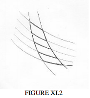
    We have specified in the above that the working substance is an ideal gas, the temperatures of source and sink being θ1 and θ2 on the ideal gas scale. Let us now not specify what the working substance is, but let us set up a system of 100 Carnot engines working in tandem, with the sink of one being the source for the next. We’ll have the sink for the coldest engine in a bucket of melting ice (0 oC) and the source for the hottest engine in a bucket of boiling water (100 oC). They will be working between isothermals and adiabats on an absolute thermodynamic scale, T, defined such that the net work done by each engine (i.e. the area of each PV loop) per cycle is the same for each of the engines. This will define the temperature on an absolute scale. It would take me a while to use the computer to do a decent drawing of 100 isotherms and 2 adiabats, so I’m going to try to make do with a hand-drawn sketch (figure X1.2) of just five isotherms, two adiabats and four linked Carnot cycles to illustrate what I am trying to describe.

    We suppose that the efficiency of such a Carnot engine depends solely on the temperature of source and sink:

    \[Q_{1} / Q_{2}=f\left(T_{1}, T_{2}\right).\]

    We are making no assumption about the form of this function, which is completely arbitrary. We are free to define it in any manner that is useful to us in our attempt to define an absolute temperature scale.
    Screen Shot 2019-07-04 at 6.51.57 PM.png

    Let us consider two adjacent engines, one working between temperatures T1 and T2, and the other working between temperatures T2 and T3. We have:

    \[ {l}{Q_{1} / Q_{2}=f\left(T_{1}, T_{2}\right)}\]

    \[{Q_{2} / Q_{3}=f\left(T_{2}, T_{3}\right)}\]

    and for the pair as a whole considered as a single engine,

    \[ Q_{1} / Q_{3}=f\left(T_{1}, T_{3}\right).\]

    From these we find that

    \[ f\left(T_{1}, T_{2}\right)=\frac{f\left(T_{1}, T_{3}\right)}{f\left(T_{2}, T_{3}\right)}.\]

    This can be only if T3 cancels from the right hand side, so that

    \[ f\left(T_{1}, T_{2}\right)=\frac{\phi\left(T_{1}\right)}{\phi\left(T_{2}\right)}.\]

    That is,

    \[ \frac{Q_{1}}{Q_{2}}=\frac{\phi\left(T_{1}\right)}{\phi\left(T_{2}\right)}.\]

    And since φ is a completely arbitrary function that we can choose at our pleasure to define an absolute scale, we choose

    \[ \frac{Q_{1}}{Q_{2}}=\frac{T_{1}}{T_{2}}.\]

    And, with this choice, the absolute thermodynamic temperature scale is identical with the ideal gas temperature scale. Equation 11.2.17 also implies that entropy in = entropy out. Entropy is conserved around the complete cycle. Entropy is a function of state.

    In Sections 11.3 to 11.5 I give examples of some other cycles. These are largely for reference, and readers who wish to continue without interruption with the theoretical development of the subject can safely skip these and move on to Sections 11.7 and 11.8.


    This page titled 11.2: The Carnot Cycle is shared under a CC BY-NC license and was authored, remixed, and/or curated by Jeremy Tatum.

    • Was this article helpful?