4.3: Accelerated motion when the velocity vector changes direction

One key difference with one dimensional motion is that, in two dimensions, it is possible to have an acceleration even when the speed is constant. Recall, the acceleration vector is defined as the time derivative of the velocity vector (Equation 4.1.4). This means that if the velocity vector changes with time, then the acceleration vector is non-zero. If the length of the velocity vector (speed) is constant, it is still possible that the direction of the velocity vector changes with time, and thus, that the acceleration vector is non-zero. This is, for example, what happens when an object goes around in a circle with a constant speed (the direction of the velocity vector changes).

Figure \(\PageIndex{1}\): Illustration of how the direction of the velocity vector can change when speed is constant.

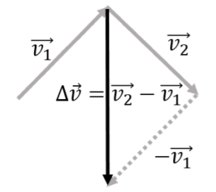
Figure \(\PageIndex{1}\) shows an illustration of a velocity vector, \(\vec v(t)\), at two different times, \(\vec v_1\) and \(\vec v_2\), as well as the vector difference, \(\Delta \vec v=\vec v_2 - \vec v_1\), between the two. In this case, the length of the velocity vector did not change with time (\(||\vec v_1||=||\vec v_2||\)). The acceleration vector is given by:

\[\begin{aligned} \vec a = \lim_{\Delta t\to 0}\frac{\Delta \vec v}{\Delta t}\end{aligned}\]

and will have a direction parallel to \(\Delta \vec v\), and a magnitude that is proportional to \(\Delta v\). Thus, even if the velocity vector does not change amplitude (speed is constant), the acceleration vector can be non-zero if the velocity vector changes direction.

Let us write the velocity vector, \(\vec v\), in terms of its magnitude, \(v\), and a unit vector, \(\hat v\), in the direction of \(\vec v\):

\[\begin{aligned} \vec v &=v_x\hat x+v_y\hat y= v \hat v\\[4pt] v&=||\vec v||=\sqrt{v_x^2+v_y^2}\\[4pt] \hat v &= \frac{v_x}{v}\hat x+\frac{v_y}{v}\hat y\\[4pt]\end{aligned}\]

In the most general case, both the magnitude of the velocity and its direction can change with time. That is, both the direction and the magnitude of the velocity vector are functions of time:

\[\begin{aligned} \vec v(t)&=v(t)\hat v(t)\end{aligned}\]

When we take the time derivative of \(\vec v(t)\) to obtain the acceleration vector, we need to take the derivative of a product of two functions of time, \(v(t)\) and \(\hat v(t)\). Using the rules for taking the derivative of a product, the acceleration vector is given by:

\[\begin{aligned} \vec a &= \frac{d}{dt}\vec v(t)= \frac{d}{dt}v(t)\hat v(t)\nonumber \end{aligned}\]

\[ \vec a = \frac{dv}{dt}\hat v(t)+v(t)\frac{d\hat v}{dt} \]

and has two terms. The first term, \(\frac{dv}{dt}\hat v(t)\), is zero if the speed is constant (\(\frac{dv}{dt}=0\)). The second term, \(v(t)\frac{d\hat v}{dt}\), is zero if the direction of the velocity vector is constant (\(\frac{d\hat v}{dt}=0\)). In general though, the acceleration vector has two terms corresponding to the change in speed, and to the change in the direction of the velocity, respectively.

The specific functional form of the acceleration vector will depend on the path being taken by the object. If we consider the case where speed is constant, then we have:

\[\begin{aligned} v(t) &= v \\[4pt] \frac{dv}{dt}&=0\\[4pt] v_x^2(t)+v_y^2(t) &=v^2 \\[4pt] \therefore v_y(t)&=\sqrt{v^2-v_x(t)^2}\end{aligned}\]

In other words, if the magnitude of the velocity is constant, then the \(x\) and \(y\) components are no longer independent (if the \(x\) component gets larger, then the \(y\) component must get smaller so that the total magnitude remains unchanged). If the speed is constant, then the acceleration vector is given by:

\[\begin{aligned} \vec a&=\frac{dv}{dt}\hat v(t)+v\frac{d\hat v}{dt}\nonumber\\[4pt] &=0 + v\frac{d}{dt}\hat v(t)\nonumber\\[4pt] &=v\frac{d}{dt}\left(\frac{v_x(t)}{v}\hat x+\frac{v_y(t)}{v}\hat y )\right)\nonumber\\[4pt] &=\frac{dv_x}{dt}\hat x + \frac{d}{dt}\sqrt{v^2-v_x(t)^2}\hat y\nonumber\\[4pt] &=\frac{dv_x}{dt}\hat x + \frac{1}{2\sqrt{v^2-v_x(t)^2}}(-2v_x(t))\frac{dv_x}{dt}\hat y\nonumber\\[4pt] &=\frac{dv_x}{dt}\hat x - \frac{v_x(t)}{\sqrt{v^2-v_x(t)^2}}\frac{dv_x}{dt}\hat y\nonumber\\[4pt] &=\frac{dv_x}{dt}\hat x - \frac{v_x(t)}{v_y(t)}\frac{dv_x}{dt}\hat y\nonumber \end{aligned}\]

\[\vec a=\frac{dv_{x}}{dt}\left( \hat x - \frac{v_{x}(t)}{v_{y}(t)}\hat y \right)\]

where most of the algebra that we did was to separate the \(x\) and \(y\) components of the acceleration vector, and we used the Chain Rule to take the derivative of the square root. The resulting acceleration vector is illustrated in Figure \(\PageIndex{2}\) along with the velocity vector¹.

Figure \(\PageIndex{2}\): Illustration that the acceleration vector is perpendicular to the velocity vector if speed is constant.

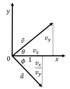
The velocity vector has components \(v_x\) and \(v_y\), which allows us to calculate the angle, \(\theta\) that it makes with the \(x\) axis:

\[\begin{aligned} \tan(\theta)=\frac{v_y}{v_x}\end{aligned}\]

Similarly, the vector that is parallel to the acceleration has components of \(1\) and \(-\frac{v_x}{v_y}\), allowing us to determine the angle, \(\phi\), that it makes with the \(x\) axis:

\[\begin{aligned} \tan(\phi)=\frac{v_x}{v_y}\end{aligned}\]

Note that \(\tan(\theta)\) is the inverse of \(\tan(\phi)\), or in other words, \(\tan(\theta)=\cot(\phi)\), meaning that \(\theta\) and \(\phi\) are complementary and thus must sum to \(\frac{\pi}{2}\) (90). This means that the acceleration vector is perpendicular to the velocity vector if the speed is constant and the direction of the velocity changes.

In other words, when we write the acceleration vector, we can identify two components, \(\vec a_{\parallel}(t)\) and \(\vec a_{\perp}(t)\):

\[\begin{aligned} \vec a&=\frac{dv}{dt}\hat v(t)+v(t)\frac{d\hat v}{dt}\\[4pt] &=\vec a_{\parallel}(t) + \vec a_{\perp}(t)\\[4pt] \therefore \vec a_{\parallel}(t)&=\frac{dv}{dt}\hat v(t)\\[4pt] \therefore \vec a_{\perp}(t)&=v\frac{d\hat v}{dt}=\frac{dv_x}{dt} \left(\hat x - \frac{v_x(t)}{v_y(t)}\hat y\right)\end{aligned}\]

where \(\vec a_{\parallel}(t)\) is the component of the acceleration that is parallel to the velocity vector, and is responsible for changing its magnitude, and \(\vec a_{\perp}(t)\), is the component that is perpendicular to the velocity vector and is responsible for changing the direction of the motion.

Exercise \(\PageIndex{1}\)

A satellite moves in a circular orbit around the Earth with a constant speed. What can you say about its acceleration vector?

1. It has a magnitude of zero.
2. It is perpendicular to the velocity vector.
3. It is parallel to the velocity vector.
4. It is in a direction other than parallel or perpendicular to the velocity vector.

Answer

B. If the speed does not change, the acceleration cannot act in the same direction as the motion.

Footnotes

1. Rather, it is a vector parallel to the acceleration vector that is illustrated, as the factor of \(\frac{dv_{x}}{dt}\) was omitted (as you recall, multiplying by a scalar only changes the length, not the direction)