6.2: Linear motion

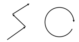
We can describe the motion of an object whose velocity vector does not continuously change direction as “linear” motion. For example, an object that moves along a straight line in a particular direction, then abruptly changes direction and continues to move in a straight line can be modeled as undergoing linear motion over two different segments (which we would model individually). An object moving around a circle, with its velocity vector continuously changing direction, would not be considered to be undergoing linear motion. For example, paths of objects undergoing linear and non-linear motion are illustrated in Figure $\PageIndex{1}$.

Figure $\PageIndex{1}$: (Left:) Displacement vectors for an object undergoing three segments that can each be modeled as linear motion. (Right:) Path of an object whose velocity vector changes continuously and cannot be considered as linear motion.

When an object undergoes linear motion, we always model the motion of the object over straight segments separately. Over one such segment, the acceleration vector will be co-linear with the displacement vector of the object (parallel or anti-parallel - note that the acceleration can change direction as it would from a spring force, but will always be co-linear with the displacement).

Example $\PageIndex{1}$

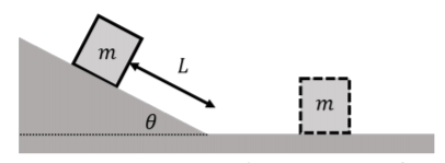
A block of mass $m$ is placed at rest on an incline that makes an angle $\theta$ with respect to the horizontal, as shown in Figure $\PageIndex{2}$. The block is nudged slightly so that the force of static friction is overcome and the block starts to accelerate down the incline. At the bottom of the incline, the block slides on a horizontal surface.

The coefficient of kinetic friction between the block and the incline is $\mu_{k1}$, and the coefficient of kinetic friction between the block and horizontal surface is $\mu_{k2}$. If one assumes that the block started at rest a distance $L$ from the bottom of the incline, how far along the horizontal surface will the block slide before stopping?

Figure $\PageIndex{2}$: A block slides down an incline before sliding on a flat surface and stopping.

Solution

We can identify that this is linear motion that we can break up into two segments: (1) the motion down the incline, and (2), the motion along the horizontal surface. We will thus identify the forces, draw the free-body diagram for the block, and use Newton’s Second Law twice, once for each segment.

It is often useful to describe the motion in words to help us identify the steps required in building a model for the block. In this case we could say that:

1. The block slides down the incline and accelerates in the direction of motion. By identifying the forces and applying Newton’s Second Law, we can determine its acceleration which will be parallel to the incline.
2. The block will reach a certain speed at the bottom of the incline, which we can determine from kinematics by knowing that the block traveled a distance $L$, with a known acceleration and that it started at rest.
3. The block will decelerate along the horizontal surface. Again, by identifying the forces and using Newton’s Second Law, we will be able to determine the acceleration of the block.
4. The block will stop after having traveled an unknown distance, which we can find by using kinematics and knowing the acceleration of the block as well as its initial velocity at the bottom of the incline.

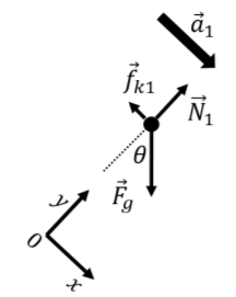
Our first step is thus to identify the forces on the block while it is on the incline. These are:

1. $\vec F_{g}$, its weight.
2. $\vec N_1$, a normal force exerted by the incline.
3. $\vec f_{k1}$, a force of kinetic friction exerted by the incline. The force is opposite of the direction of motion, and has a magnitude given by $f_{k1}=\mu_{k1}N_1$.

These are shown on the free-body diagram in Figure $\PageIndex{3}$. As usual, we drew the acceleration, $\vec a_1$, on the free-body diagram, and chose the direction of the $x$ axis to be parallel to the acceleration.

Figure $\PageIndex{3}$: Free-body diagram for the block when it is on the incline.

Writing out the $x$ component of Newton’s Second Law, and using the fact that the acceleration is in the $x$ direction ($\vec a=a_1\hat x$):

$$\begin{aligned} \sum F_x = F_g\sin\theta - f_{k1} &= ma_1\\[4pt] \therefore mg\sin\theta - \mu_{k1} N_1 &= ma_1\end{aligned}$$

where we expressed the magnitude of the kinetic force of friction in terms of the normal force exerted by the plane, and the weight in terms of the mass and gravitational field, $g$. The $y$ component of Newton’s Second Law can be written:

$$\begin{aligned} \sum F_y = N_1-F_g\cos\theta &= 0\\[4pt] \therefore N_1 = mg\cos\theta\end{aligned}$$

which we used to express the normal force in terms of the weight. We can use this expression for the normal force by substituting it into the equation we obtained from the $x$ component to find the acceleration along the incline:

$$\begin{aligned} mg\sin\theta - \mu_{k1} N_1 &= ma_1\\[4pt] mg\sin\theta - \mu_{k1} mg\cos\theta&= ma_1\\[4pt] \therefore a_1 &= g(\sin\theta-\mu_{k1}\cos\theta)\end{aligned}$$

Now that we know the acceleration down the incline, we can easily find the velocity at the bottom of the incline using kinematics. We choose the origin of the $x$ axis to be zero where the block started ($x_0=0$), so that the block is at position $x=L$ at the bottom of the incline. Using kinematics, we can find the speed, $v$, given that the initial speed, $v_0=0$:

$$\begin{aligned} v^2-v_0^2&=2a_1(x-x_0)\\[4pt] v^2&=2a_1L\\[4pt] \therefore v &= \sqrt{2a_1L}\\[4pt] &=\sqrt{2Lg(\sin\theta-\mu_{k1}\cos\theta)}\end{aligned}$$

We can now proceed to build a model for the second segment. We first identify the forces on the block when it is on the horizontal surface; these are:

1. $\vec F_{g1}$, its weight.
2. $\vec N_2$, a normal force exerted by the horizontal surface. This is in general different than the normal force exerted when the block was on the inclined plane.
3. $\vec f_{k2}$, a force of kinetic friction exerted by the horizontal surface. The force is opposite of the direction of motion, and has a magnitude given by $f_{k2}=\mu_{k2}N_2$.

The forces are illustrated by the free-body diagram in Figure $\PageIndex{4}$, where we showed the acceleration vector, $\vec a_2$, which we determined to be to the left since the block is decelerating. We also chose an $xy$ coordinate system such that the $x$ axis is anti-parallel to the acceleration, so that the motion is in the positive $x$ direction (and the acceleration in the negative $x$ direction).

Figure $\PageIndex{4}$: Free-body diagram for the block when it is sliding along the horizontal surface. We (arbitrarily) chose the positive $x$ direction to be in the direction of motion and anti-parallel to the acceleration. We could easily have chosen the opposite direction.

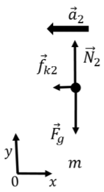
Writing out the $x$ component of Newton’s Second Law:

$$\begin{aligned} \sum F_x = -f_{k2} &= -ma_2\\[4pt] \therefore \mu_{k2}N_2 &= ma_2\end{aligned}$$

where we expressed the force of kinetic friction using the normal force. We have to be careful here with the sign of the acceleration; the equation that we wrote implies that $a_2$ is a positive number, since $\mu_{k2}$ is positive and $N_2$ is also positive (it is the magnitude of the normal force). $a_2$ is the magnitude of the acceleration, and we included the fact that the acceleration points in the negative $x$ direction when we put a negative sign in the first line. The $x$ component of the acceleration is $-a_2$, and the vector is given by $\vec a_2=-a_2\hat x$.

The $y$ component of Newton’s Second Law will allow us to find the normal force:

$$\begin{aligned} \sum F_y = N_2 -F_g &=0\\[4pt] \therefore N_2 = mg\end{aligned}$$

which we can substitute back into the $x$ equation to find the magnitude of the acceleration along the horizontal surface:

$$\begin{aligned} ma_2 &=\mu_{k2}N_2 \\[4pt] \therefore a_2&=\mu_{k2}g\end{aligned}$$

Now that we have found the acceleration along the horizontal surface, we can use kinematics to find the distance that the block travelled before stopping. We choose the origin of the $x$ axis to be the bottom of the incline ($x_0=0$), the acceleration is negative $a_x = -a_2 = -mu_{k2}g$, the final speed is zero, $v=0$, and the initial speed, $v_0$ is given by our model for the first segment. Using one of the kinematic equations:

$$\begin{aligned} v^2-v_0^2&=2(-a_2)(x-x_0)\\[4pt] v_0^2&=2a_2x\\[4pt] \therefore x &=\frac{1}{2a_2}v_0^2\\[4pt] &=\frac{1}{2\mu_{k2}g}2Lg(\sin\theta-\mu_{k1}\cos\theta)\\[4pt] \therefore x&=\frac{(\sin\theta-\mu_{k1}\cos\theta)}{\mu_{k2}}L\end{aligned}$$

Discussion

The model for the distance $x$ that it takes the block to stop makes sense because:

• All of the terms in the fraction are dimensionless, so the value of $x$ will have the same dimension as $L$.
• If we make $L$ bigger, then $x$ will be bigger (if we release the block from higher up on the incline, it will have more time to accelerate and will slide further before stopping).
• If we make $\mu_{k1}$ bigger, then $x$ will be smaller: if we increase friction on the incline, the block will have a smaller acceleration and smaller speed at the bottom.
• If we increase the friction with the horizontal plane (increase $\mu_{k2}$), then $x$ will be reduced (it won’t slide as far if there is more friction on the horizontal plane).
• If we increase $\theta$, the numerator will be larger, so $x$ will increase (the block will accelerate more down a steeper incline and end up further).

Exercise $\PageIndex{1}$

A present is placed at rest on a plane that is inclined, at a distance $L$ from the bottom of the incline, much like the box in Example 6.2.1 above. At the bottom of the incline, the box is determined to have a speed $v$. If the box is instead released from a distance of $4L$ from the bottom of the incline, what will its speed at the bottom of the incline be?

1. $v$
2. $2v$
3. $4v$
4. it depends on the coefficient of friction between the present and the plane.

Answer

B.

Modeling situations where forces change magnitude

So far, the models that we have considered involved forces that remained constant in magnitude. In many cases, the forces exerted on an object can change magnitude and direction. For example, the force exerted by a spring changes as the spring changes length or the force of drag changes as the object changes speed. In these case, even if the object undergoes linear motion, we need to break up the motion into many small segments over which we can assume that the forces are constant. If the forces change continuously, we will need to break up the motion into an infinite number of segments and use calculus.

Consider the block of mass $m$ that is shown in Figure $\PageIndex{5}$, which is sliding along a frictionless horizontal surface and has a horizontal force $\vec F(x)$ exerted on it. The force has a different magnitude in the three segments of length $\Delta x$ that are shown. If the block starts at position $x=x_0$ axis with speed $v_0$, we can find, for example, its speed at position $x_3=3\Delta x$, after the block traveled through the three segments.

Figure $\PageIndex{6}$: A block being pushed along a frictionless horizontal surface with a force that changes.

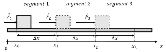
The horizontal force, $\vec F$, exerted on the block can be written as:

$$\begin{aligned} \vec F (x)= \begin{cases} F_1\hat x & x<\Delta x \quad \text{(segment 1)}\\[4pt] F_2\hat x & \Delta x \leq x< 2\Delta x \quad \text{(segment 2)}\\[4pt] F_3\hat x & 2\Delta x \leq x\quad \text{(segment 3)} \end{cases}\end{aligned}$$

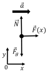
as it depends on the location of the block. To find the speed of the block at the end of the third segment, we can model each segment separately. The forces exerted on the block are the same in each segment:

1. $\vec F_g$, its weight, with magnitude $mg$.
2. $\vec N$, a normal force exerted by the ground.
3. $\vec F(x)$, an applied force that changes magnitude with position and is different in the three different segments.

The forces are illustrated in the free-body diagram show in Figure $\PageIndex{7}$.

Figure $\PageIndex{6}$.

Newton’s Second Law can be used to determine the acceleration of the block for each of the three segments, since the forces are constant within one segment. For all three segments, the $y$ component of Newton’s Second Law just tells us that the normal force exerted by the ground is equal in magnitude to the weight of the block. The $x$ component of Newton’s Second Law gives the acceleration:

$$\begin{aligned} \sum F_x = F_i = ma_i\end{aligned}$$

where we have used the index $i$ to indicate which segment the block is in ($i$ can be 1, 2 or 3). The acceleration of the block in segment $i$ is given by:

$$\begin{aligned} a_i = \frac{F_i}{m}\end{aligned}$$

If the speed of the block is $v_0$ at the beginning of segment 1 ($x=x_0$), we can find its speed at the end of segment 1 ($x=x_1$), $v_1$, using kinematics and the fact that the acceleration in segment 1 is $a_1$:

$$\begin{aligned} v_1^2-v_0^2 &= 2a_1(x_1 - x_0)\\[4pt] v_1^2 &=v_0^2+ 2a_1\Delta x\\[4pt] \therefore v_1^2 &=v_0^2+2\frac{F_1}{m}\Delta x\end{aligned}$$

We can now easily find the speed at the end of segment 2 ($x=x_2$), $v_2$, since we know the speed at the beginning of segment 2 ($x_1$,$v_1$) and the acceleration $a_2$:

$$\begin{aligned} v_2^2 -v_1^2 &= 2a_2(x_2 - x_1)\\[4pt] \therefore v_2^2 &= v_1^2 + 2a_2\Delta x\\[4pt] &=v_0^2+ 2\frac{F_1}{m}\Delta x + 2\frac{F_2}{m}\Delta x\end{aligned}$$

It is easy to show that the speed at the end of the third segment is:

$$\begin{aligned} v_3^2 = v_0^2+ 2\frac{F_1}{m}\Delta x + 2\frac{F_2}{m}\Delta x +2\frac{F_3}{m}\Delta x\end{aligned}$$

If there were $N$ segments, with the force being different in each segment, we could use the summation notation to write:

$$\begin{aligned} v_N^2 &= v_0^2 + 2\sum_{i=1}^{i=N} \frac{F_i}{m}\Delta x\end{aligned}$$

Finally, if the magnitude of the force varied continuously as a function of $x$, $\vec F(x)$, we would model this by taking segments whose length, $\Delta x$, tends to zero (and we would need an infinite number of such segments). For example, if we wanted to know the speed of the object at position $x=X$ along the $x$ axis, with a force that was given by $\vec F(x)=F(x)\hat x$, if the object started at position $x_0$ with speed $v_0$, we would take the following limit:

$$\begin{aligned} v^2 = v_0^2 + \lim_{\Delta x \to 0} 2\sum_{i=1}^{i=N} \frac{F(x)}{m}\Delta x\end{aligned}$$

where $\Delta x = \frac{X}{N}$ so that as $\Delta x\to 0$, $N\to\infty$. Of course, integrals are the exact tool that allow us to evaluate the sum in this limit:

$$\begin{aligned} \lim_{\Delta x \to 0} 2\sum_{i=1}^{i=N} \frac{F_i}{m}\Delta x =2 \int_{x_0}^{X}\frac{F(x)}{m}dx \end{aligned}$$

and the speed at position $x=X$ is given by:

$$\begin{aligned} v^2 = v_0^2 + 2 \int_{x_0}^{X}\frac{F(x)}{m}dx \end{aligned}$$

Naturally, we can find the above result starting directly from calculus. If the component of the (net) force in the $x$ direction is given by $F(x)$, then the acceleration is given by $a(x) = \frac{F(x)}{m}$. The velocity is related to the acceleration:

$$\begin{aligned} a(x) &= \frac{dv}{dt}\\[4pt] \therefore dv &= a(x)dt\\[4pt]\end{aligned}$$

We cannot simply integrate the last equation to find that $v=\int a(x)dt$ because the acceleration is given as a function of position, $a(x)$, and not a function of time, $t$. Thus, we cannot simply take the integral over $t$ and must instead “change variables” to take the integral over $x$. $x$ and $t$ are related through velocity:

$$\begin{aligned} v &= \frac{dx}{dt}\\[4pt] \therefore dt &= \frac{1}{v}dx\end{aligned}$$

We can thus write:

$$\begin{aligned} dv &= a(x)dt = a(x)\frac{1}{v}dx \\[4pt]\end{aligned}$$

The equation above is called a “separable differential equation”, which can also be written:

$$\begin{aligned} \frac{dv}{dx}=\frac{1}{v}a(x)\end{aligned}$$

This is called a differential equation because it relates the derivative of a function (the derivative of $v$ with respect to $x$, on the left) to the function itself ($v$ appears on the right as well). The differential equation is “separable”, because we can separate out all of the quantities that depend on $v$ and on $x$ on different sides of the equation:

$$\begin{aligned} vdv = a(x)dx\end{aligned}$$

This last equation says that $vdv$ is equal to $a(x)dx$. Remember that $dx$ is the length of a very small segment in $x$, and that $dv$ is the change in velocity over that very small segment. Since the terms on the left and right are equal, if we sum (integrate) the quantity $vdv$ over many segments, that sum must be equal to the sum (integral) of the quantity $a(x)dx$ over the same segments. Let us choose those segment such that for the beginning of the first interval the position and speed are $x_0$ and $v_0$, respectively, and the position and speed at the end of the last segment are $X$ and $V$, respectively. We then must have that:

$$\begin{aligned} \int_{v_0}^{V}vdv&=\int_{x_0}^{X}a(x)dx\\[4pt] \frac{1}{2}V^2 - \frac{1}{2}v_0^2 &= \int_{x_0}^{X}a(x)dx\\[4pt] \therefore V^2 &= v_0^2 + 2\int_{x_0}^{X}a(x)dx\\[4pt]\end{aligned}$$

which is the same as we found earlier. If the acceleration is constant, we recover our formula from kinematics:

$$\begin{aligned} V^2 &= v_0^2+ 2\int_{x_0}^{X}adx\\[4pt] &=v_0^2+ 2a(X-x_0)\\[4pt] \therefore V^2- v_0^2 &= 2a(X-x_0)\end{aligned}$$

Example $\PageIndex{2}$

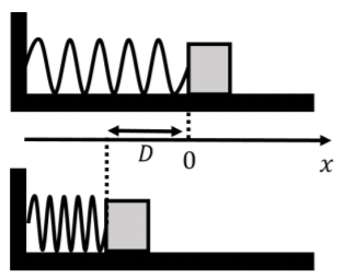
A block of mass $m$ can slide freely along a frictionless surface. A horizontal spring, with spring constant, $k$, is attached to a wall on one end, while the other end can move freely, as shown in Figure $\PageIndex{8}$. A coordinate system is defined such that the $x$ axis is horizontal and the free end of the spring is at $x=0$ when the spring is at rest. The block is pushed against the spring so that the spring is compressed by a distance $D$. The block is then released. What speed will the block have when it leaves the spring?

Figure $\PageIndex{8}$: A block is launched along a frictionless surface by compressing a spring by a distance $D$. The top panel shows the spring when at rest, and the bottom panel shows the spring compressed by a distance $D$ just before releasing the block.

Solution

As you recall, the force exerted by a spring depends on the compression or extension of the spring and is given by Hooke’s Law:

$$\begin{aligned} \vec F(x) = -kx\hat x\end{aligned}$$

where $x$ is the position of the free end of the spring and $x=0$ corresponds to the spring being at rest. In our case, when the edge of the block is located at $x_0=-D$ (the spring is compressed), the force is thus in the positive $x$ direction (since $x_0$ is a negative number).

The forces on the block are:

1. $\vec F_g$, its weight, with magnitude $mg$.
2. $\vec N$, a normal force exerted by the ground.
3. $\vec F(x)$, the spring force.

Since the block is not moving vertically, the magnitude of the normal force must equal the weight $N=mg$, since these are the only forces with components in the vertical direction. The $x$ component of Newton’s Second Law gives us the acceleration of the block (which depends on $x$):

$$\begin{aligned} \sum F_x = -kx &= ma(x)\\[4pt] \therefore a(x)&=-\frac{k}{m}x\end{aligned}$$

Again, recall that if $x$ is negative, then the acceleration will be in the positive direction. Since this scenario is exactly the same that we described above in the text, namely a force that varies continuously with position, we can apply the formula that we found earlier for determining the velocity after a varying force has been applied from position $x=x_0$ to position $x=X$:

$$\begin{aligned} V^2 &= v_0^2 + 2\int_{x_0}^{X}a(x)dx\end{aligned}$$

$V$ is the final speed that we would like to find, $v_0=0$ because the block starts at rest, and $x_0=-D$ is the starting position of the block. $X$ is the position along the $x$ axis where the block leaves the spring.

We have to think a little about what the value of $X$ should be: when the spring is compressed and the block accelerating, the spring is pushing the block in the positive $x$ direction. Once the block reaches $x=0$ the spring would want to pull the block backwards, but since it is not attached to the block, it stops exerting a force on the block at that point. The block thus leaves the spring at $x=0$, so that the final position is $X=0$. The speed of the block when it leaves the spring is thus:

$$\begin{aligned} V^2 &= v_0^2 + 2\int_{x_0}^{X}a(x)dx\\[4pt] &= 0 + 2\int_{-D}^{0}a(x)dx\\[4pt] &= 2\int_{-D}^{0}-\frac{k}{m}xdx\\[4pt] &= 2\left[ - \frac{k}{m}\frac{1}{2}x^2\right]_{-D}^{0}\\[4pt] &= \frac{k}{m}D^2\\[4pt] \therefore V &= \sqrt{\frac{k}{m}}D\end{aligned}$$

Discussion

This model for the speed of the block when it leaves the spring makes sense because:

• The dimension for the expression for $V$ is correct (you should check this!).
• If the spring is compressed more (bigger value of $D$), then the speed will be higher.
• If the mass is bigger (more inertia), then the final speed will be lower.
• If the spring is stiffer (bigger value of $k$), then the final speed will be higher.

If you have studied physics before, you may have realized that the speed is easily found by conservation of energy:

$$\begin{aligned} \frac{1}{2}mV^2=\frac{1}{2}kD^2\end{aligned}$$

which gives the same value for $V$. As we will see in a later chapter, kinetic and potential energy are defined as they are, precisely because it makes using conservation of energy equivalent to using forces as we just did.

Example $\PageIndex{3}$

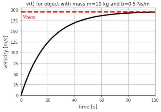
An object of mass $m$ is released from rest out of a helicopter. The drag (air-resistance) on the object can be modeled as having a magnitude given by $bv$, where $v$ is the speed of the object and $b$ is a constant of proportionality. How does the velocity of the object depend on time?

Solution

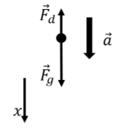
As the object falls through the air, the forces exerted on the object are:

1. $F_g$, its weight, with magnitude $mg$, exerted downwards.
2. $F_d$, the force of drag, with magnitude $bv$, exerted upwards.

Since the object will fall in a straight line, this is a one-dimensional problem, and we can choose the $x$ axis to be vertical, with positive $x$ pointing downwards, and the origin located where the object was released. The object will thus have a positive acceleration and move in the positive $x$ direction with this choice of coordinate system. This is illustrated in the free-body diagram in Figure $\PageIndex{9}$.

Figure $\PageIndex{9}$: Free-body diagram for a block free-falling with drag.

Newton’s Second Law for the object gives:

$$\begin{aligned} \sum F_x = F_g - F_d &= ma\\[4pt] mg - bv &= ma\\[4pt] \therefore a &= g-\frac{b}{m}v \end{aligned}$$

In this case, the acceleration depends explicitly on velocity rather than position, as we had before. However, we can use the same methodology to find how the velocity changes with time. First, we can note that the acceleration is zero if:

$$\begin{aligned} g-\frac{b}{m}v &=0\\[4pt] \therefore v = \frac{mg}{b}\end{aligned}$$

That is, once the object reaches a speed of $v_{term}=mg/b$, it will stop accelerating, i.e. it will reach “terminal velocity”. Note that this is the same condition as requiring that the drag force ($bv$) have the same magnitude as the weight ($mg$).

Writing the acceleration as $a=\frac{dv}{dt}$, we can write:

$$\begin{aligned} \frac{dv}{dt} &= \left(g-\frac{b}{m}v \right)\end{aligned}$$

which again, is a separable differential equation, in which we can write the terms that depend on $v$ and those that depend on $t$ on separate sides of the equal sign:

$$\begin{aligned} \frac{dv}{g-\frac{b}{m}v}&= dt\\[4pt] \frac{dv}{v-\frac{mg}{b}}&= -\frac{b}{m}dt\\[4pt]\end{aligned}$$

where we re-arranged the equation in the second line so that it would be easier to integrate in the next step. We can find the velocity, $v(t)$, at some time, $t$, by stating that $v=0$ at $t=0$ and taking the integrals (sum) on both sides. Again, we are modelling the motion as being made up of a large number of very small segments where the quantities on both sides of the equation are the same. Thus, if we sum (integrate) those quantities over all of the same segments, the left and right hand side of the equations will still be equal to each other:

$$\begin{aligned} \int_0^{v(t)}\frac{dv}{v-\frac{mg}{b}} &= -\int_0^t\frac{b}{m} dt\\[4pt] \left[\ln\left(v-\frac{mg}{b} \right)\right]_0^{v(t)} &=-\frac{b}{m}t\\[4pt] \ln\left(v(t)-\frac{mg}{b} \right)-\ln\left(-\frac{mg}{b} \right)&=-\frac{b}{m}t\\[4pt] \ln\left( \frac{v(t)-\frac{mg}{b}}{-\frac{mg}{b}} \right)&=-\frac{b}{m}t\\[4pt]\end{aligned}$$

where, in the last line, we used the property that $\ln(a)-\ln(b)=\ln(a/b)$. By taking the exponential on either side of the equation ($e^{\ln(x)}=x$), we can find an expression for the velocity as a function of time:

$$\begin{aligned} \frac{v(t)-\frac{mg}{b}}{-\frac{mg}{b}} &= e^{-\frac{b}{m}t}\\[4pt] v(t)-\frac{mg}{b} &= -\frac{mg}{b}e^{-\frac{b}{m}t}\\[4pt] \therefore v(t) &= \frac{mg}{b}-\frac{mg}{b}e^{-\frac{b}{m}t}\\[4pt] &=\frac{mg}{b}\left(1-e^{-\frac{b}{m}t}\right)\end{aligned}$$

Discussion

This equation tells us that the velocity increases as a function of time, but the rate of increase decreases exponentially with time. At time $t=0$, the velocity is zero, as expected. As $t$ approaches infinity, $v$ approaches, $\frac{mg}{b}$, which is the terminal velocity. The time dependence of the velocity is illustrated in Figure $\PageIndex{10}$.

Figure $\PageIndex{10}$: Velocity as a function of time for an object of mass $m = 10\text{ kg}$ which is freefalling from rest with a drag coefficient $b = 0.5\text{ Ns/m}$.