
2.3: Making Measurements


- Last updated
- Mar 28, 2024
- Save as PDF
( \newcommand{\kernel}{\mathrm{null}\,}\)
Having introduced some tools for the modeling aspect of physics, we now address the other side of physics, namely performing experiments. Since the goal of developing theories and models is to describe the real world, we need to understand how to make meaningful measurements that test our theories and models.
Suppose that we wish to test Chloe’s theory of falling objects from Chapter 1:
t=k√x
which states that the time, t, for any object to fall a distance, x, near the surface of the Earth is given by the above relation. The theory assumes that Chloe’s constant, k, is the same for any object falling any distance on the surface of the Earth.
One possible way to test Chloe’s theory of falling objects is to measure k for different drop heights to see if we always obtain the same value. Results of such an experiment are presented in Table 2.3.1, where the time, t, was measured for a bowling ball to fall distances of x between 1 m and 5 m. The table also shows the values computed for √x and the corresponding value of k=t/√x:
| x [m] | t [s] | √x[m12] | k [sm−12] |
|---|---|---|---|
| 1.00 | 0.33 | 1.00 | 0.33 |
| 2.00 | 0.74 | 1.41 | 0.52 |
| 3.00 | 0.67 | 1.73 | 0.39 |
| 4.00 | 1.07 | 2.00 | 0.54 |
| 5.00 | 1.10 | 2.24 | 0.49 |
When looking at Table 2.3.1, it is clear that each drop height gave a different value of k, so at face value, we would claim that Chloe’s theory is incorrect, as there does not seem to be a value of k that applies to all situations. However, we would be incorrect in doing so unless we understood the precision of the measurements that we made. Suppose that we repeated the measurement multiple times at a fixed drop height of x=3 m, and obtained the values in Table 2.3.2.
| x [m] | t [s] | √x[m12] | k [sm−12] |
|---|---|---|---|
| 3.00 | 1.01 | 1.73 | 0.58 |
| 3.00 | 0.76 | 1.73 | 0.44 |
| 3.00 | 0.64 | 1.73 | 0.37 |
| 3.00 | 0.73 | 1.73 | 0.42 |
| 3.00 | 0.66 | 1.73 | 0.38 |
This simple example highlights the critical aspect of making any measurement: it is impossible to make a measurement with infinite precision. The values in Table 2.3.2 show that if we repeat the exact same experiment, we are likely to measure different values for a single quantity. In this case, for a fixed drop height, x=3 m, we obtained a spread in values of the drop time, t, between roughly 0.6 s and 1.0 s. Does this mean that it is hopeless to do science, since we can never repeat measurements? Thankfully, no! It does however require that we deal with the inherent imprecision of measurements in a formal manner.
Measurement Uncertainties
The values in Table 2.3.2 show that for a fixed experimental setup (a drop height of 3 m), we are likely to measure a spread in the values of a quantity (the time to drop). We can quantify this “uncertainty” in the value of the measured time by quoting the measured value of t by providing a “central value” and an “uncertainty”:
t=(0.76±0.15) s
where 0.76 s is called the “central value” and 0.15 s the “uncertainty” or the “error’. Note that we use the word error as a synonym for uncertainty, not “mistake”. When we present a number with an uncertainty, we mean that we are “pretty certain” that the true value is in the range that we quote. In this case, the range that we quote is that t is between 0.61 s and 0.91 s (given by 0.76 s−0.15 s and 0.76 s+0.15 s). When we say that we are “pretty sure” that the value is within the quoted range, we usually mean that there is a 68% chance of this being true and allow for the possibility that the true value is actually outside the range that we quoted. The value of 68% comes from statistics and the normal distribution.
Have you ever started writing a lab report and wondered whether or not you should describe your measurement in terms of “accuracy” or “precision”? What about describing the error in your experiment as a measure of “accuracy” or “uncertainty”?
You’re not alone! Precision, accuracy and uncertainty all relate to error, but have different meanings. To clarify these terms, I think it is useful to study them side-by-side.
- Precision refers to how close your measurements are to each other when you repeat a measurement multiple times. If the values obtained are close to one another, your measurements are precise. For example, say you were measuring the rebound height of a basketball, dropped from a fixed height. After performing the measurement multiple times, you find that the measured rebound heights are very close in value to each other. You could then report that “After repeating our measurement multiple times, the values that we obtained were very close together. Our measurements were precise!”. Of course, you have to specify what you mean by “close” (perhaps in terms of the divisions on the ruler that you used to measure rebound height).
- Accuracy measures the agreement between a measured value and its true value. If the measured value is close to the true value, your measured value is accurate. For example, say that you developed a model for the distance covered by a rock thrown with a slingshot. If you find that the measured value is close to the predicted value, you would say that your model is accurate, “Our model value was very close to the value that we measured - our model was accurate.” Again, you have to specify what you mean by “close”, usually in terms of the uncertainty on your measured value.
- Uncertainty is an estimate of the amount that a measurement will differ from a true value. In science, we aim to lower the uncertainty in our measurements, so that we can test models and theories with more precision. Let’s say that you are measuring the number of rotations of a spinning top during a certain period of time. Your measurements are close together, but have a fixed range of values. This would be an example where you could calculate the uncertainty in your measurements. It would be sensible to say “After multiple measurements, we’ve found that our values are similar and our uncertainty captures the range of values that we measured.”
Determining the central value and uncertainty
The tricky part when performing a measurement is to decide how to assign a central value and an uncertainty. For example, how did we come up with t=(0.76±0.15) s from the values in Table 2.3.2?
Determining the uncertainty and central value on a measurement is greatly simplified when one can repeat the same measurement multiple times, as we did in Table 2.3.2. With repeatable measurements, a reasonable choice for the central value and uncertainty is to use the mean and standard deviation of the measurements, respectively.
If we have N measurements of some quantity t,{t1,t2,t3,...tN}, then the mean, ¯t, and standard deviation, σt, are defined as:
¯t=1ni=N∑i=1t1=t1+t2+t3+...+tNN
σ2t=1N−1i=N∑i=1(ti−¯t)2=(t1−¯t)2+(t2−¯t)2+(t3−¯t)2+...+(tN−¯t)2N−1
σt=√σ2t
The mean is just the arithmetic average of the values, and the standard deviation, σt, requires one to first calculate the mean, then the variance (σ2t, the square of the standard deviation). You should also note that for the variance, we divide by N−1 instead of N. The standard deviation and variance are quantities that come from statistics and are a good measure of how spread out the values of t are about their mean, and are thus a good measure of the uncertainty.
Calculate the mean and standard deviation of the values for k from Table 2.3.2.
Solution
In order to calculate the standard deviation, we first need to calculate the mean of the N=5 values of k: {0.58,0.44,0.37,0.42,0.38}. The mean is given by:
¯k=0.58+0.44+0.37+0.42+0.385=0.44sm−12
We can now calculate the variance using the mean:
σ2k=14[(0.58−0.44)2+(0.44−0.44)2+(0.37−0.44)2+(0.42−0.44)2+(0.38−0.44)2]=7.3×10⁻³s2
and the standard deviation is then given by the square root of the variance:
σk=√0.0073=0.09sm−12
Using the mean and standard deviation, we would quote our value of k as:
k=(0.44±0.09)s m−12
Any value that we measure will always have an uncertainty. In the case where we can easily repeat the measurement, we should do so to evaluate how reproducible it is, and the standard deviation of those values is usually a good first estimate of the uncertainty in a value1. Sometimes, the measurements cannot easily be reproduced; in that case, it is still important to determine a reasonable uncertainty, but in this case, it usually has to be estimated. Table 2.3.3 shows a few common types of measurements and how to determine the uncertainties in those measurements.
| Type of measurement | How to determine central value and uncertainty |
|---|---|
| Repeated measurements | Mean and standard deviation |
| Single measurement with a graduated scale (e.g. ruler, digital scale, analogue meter) | Closest value and half of the smallest division |
| Counted quantity | Counted value and square root of the value |
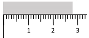
For example, we would quote the length of the grey object in Figure 2.3.1 to be L=(2.80±0.05) cm based on the rules in Table 2.3.4, since 2.8 cm is the closest value on the ruler that matches the length of the object and 0.5 mm is half of the smallest division on the ruler. Using half of the smallest division of the ruler means that our uncertainty range covers one full division. Note that it is usually better to reproduce a measurement to evaluate the uncertainty instead of using half of the smallest division, although half of the smallest division should be the lower limit on the uncertainty. That is, by repeating the measurements and obtaining the standard deviation, you should see if the uncertainty is larger than half of the of the smallest division, not smaller.
The relative uncertainty in a measured value is given by dividing the uncertainty by the central value, and expressing the result as a percent. For example, the relative uncertainty in t=(0.76±0.15) s is given by 0.15/0.76=20%. The relative uncertainty gives an idea of how precisely a value was determined. Typically, a value above 10% means that it was not a very precise measurement, and we would generally consider a value smaller than 1% to correspond to quite a precise measurement.
Random and systematic sources of error/uncertainty
It is important to note that there are two possible sources of uncertainty in a measurement. The first is called “statistical” or “random” and occurs because it is impossible to exactly reproduce a measurement. For example, every time you lay down a ruler to measure something, you might shift it slightly one way or the other which will affect your measurement. The important property of random sources of uncertainty is that if you reproduce the measurement many times, these will tend to cancel out and the mean can usually be determined to high precision with enough measurements.
The other source of uncertainty is called “systematic”. Systematic uncertainties are much more difficult to detect and to estimate. One example would be trying to measure something with a scale that was not properly tarred (where the 0 weight was not set). You may end up with very small random errors when measuring the weights of object (very repeatable measurements), but you would have a hard time noticing that all of your weights were offset by a certain amount unless you had access to a second scale. Some common examples of systematic uncertainties are: incorrectly calibrated equipment, parallax error when measuring distance, reaction times when measuring time, effects of temperature on materials, etc.
As a reminder, we want to emphasized the difference between “error” and “mistake” in the context of making measurements. “Uncertainty” or “error” in a measurement comes from the fact that it is impossible to measure anything to infinite accuracy. A “mistake” also affects a measurement, but is preventable. If a “mistake” occurs in physics, the experiment is generally re-done and the previous data are discarded. The term “human error” should never be used in a lab report as it implies that a mistake was made. Instead, if you think that you measured time imprecisely, for example, refer to human reaction time, not “human error”.
Table 2.3.4 shows examples of sources of error that students often call “human error” but that should be instead described more precisely.
| Situation | Source of Error |
|---|---|
| While taking measurements, your line of sight was not completely parallel to the measuring device. | This is parallax error - a type of systematic error. |
| You incorrectly performed calculations. | Mistake! Redo the calculations. |
| A draft of wind in the lab slightly altered the direction of your ball rolling down an incline. | This is an environmental effect/error - it could be random or systematic, depending on whether it always had the same effect. |
| Your hand slipped while holding the ruler - the object was measured to be twice its original size! | Mistake! Redo this experiment and discard the data. |
| When timing an experiment, you don’t hit the ”STOP” button exactly when the experiment stops. | Reaction time error - usually a systematic error (time is usally measured longer than it is). |
Propagating uncertainties
Going back to the data in Table 2.3.2, we found that for a known drop height of x=3 m, we measured different values of the drop time, which we found to be t=(0.76±0.15) s (using the mean and standard deviation). We also calculated a value of k corresponding to each value of t, and found k=(0.44±0.09)s m−12 (Example 2.3.1).
Suppose that we did not have access to the individual values of t, but only to the value of t = (0.76 ± 0.15) s with uncertainty. How do we calculate a value for k with uncertainty? In order to answer this question, we need to know how to “propagate” the uncertainties in a measured value to the uncertainty in a value derived the measured value. We briefly present different methods for propagating uncertainties, before advocating for the use of computers to do the calculations for you.
1. Estimate using relative uncertainties
The relative uncertainty in a measurement gives us an idea of how precisely a value was determined. Any quantity that depends on that measurement should have a precision that is similar; that is, we expect the relative uncertainty in k to be similar to that in t. For t, we saw that the relative uncertainty was approximately 20%. If we take the central value of k to be the central value of t divided by √x, we find:
k=(0.76 s√(3m)=0.44sm−12
Since we expect the relative uncertainty in k to be approximately 20%, then the absolute uncertainty is given by:
σk=(0.2)k=0.09sm−12
which is close to the value obtained by averaging the five values of k in Table 2.3.2.
2. The Min-Max method
A pedagogical way to determine k and its uncertainty is to use the “Min-Max method”. Since k=t/√x, k will be the biggest when t is the biggest, and the smallest when t is the smallest. We can thus determine “minimum” and “maximum” values of k corresponding to the minimum value of t, tmin=0.61 s and the maximum value of t,tmax=0.91 s:
kmin=tmin√x=0.61√(3m)=0.35sm−12kmax=tmax√x=0.91s√(3m)=0.53sm−12
This gives us the range of values of k that correspond to the range of values of t. We can choose the middle of the range as the central value of k and half of the range as the uncertainty:
¯k=12(kmin+kmax)=0.44sm−12σk=12(kmax−kmin)=0.09sm−12∴
which, in this case, gives the same value as that obtained by averaging the individual values of k. While the Min-Max method is useful for illustrating the concept of propagating uncertainties, we usually do not use it in practice as it tends to overestimate the uncertainty.
3. The derivative method
In the example above, we assumed that the value of x was known precisely (and we chose 3 m), which of course is not realistic. Let us suppose that we have measured x to within 1 cm so that x = (3.00 ± 0.01) m. The task is now to calculate k = \frac{t}{\sqrt{x}} when both x and t have uncertainties.
The derivative method lets us propagate the uncertainty in a general way, so long as the relative uncertainties on all quantities are “small” (less than 10-20%). If we have a function, F(x, y) that depends on multiple variables with uncertainties (e.g. x±σ_{x}, y ±σ_{y}), then the central value and uncertainty in F(x, y) are given by:
\overline{F}=F(\overline{x}, \overline{y})
\sigma_{F}=\sqrt{\left(\frac{∂F}{∂x}\sigma_{x} \right)^{2}+\left( \frac{∂F}{∂y}\sigma_{y} \right)^{2}}
That is, the central value of the function F is found by evaluating the function at the central values of x and y. The uncertainty in F, σ_{F}, is found by taking the quadrature sum of the partial derivatives of F evaluated at the central values of x and y multiplied by the uncertainties in the corresponding variables that F depends on. The uncertainty will contain one term in the sum per variable that F depends on.
In appendix D, we will show you how to calculate this easily with a computer, so do not worry about getting comfortable with partial derivatives (yet!). Note that the partial derivative, \frac{∂F}{∂x}, is simply the derivative of F(x,y) relative to x evaluated as if y were a constant. Also, when we say “add in quadrature”, we mean square the quantities, add them, and then take the square root (same as you would do to calculate the hypotenuse of a right-angle triangle).
Use the derivative method to evaluate k = \frac{t}{\sqrt{x}} for x = (3.00 ± 0.01) m and t = (0.76 ± 0.15) s.
Solution
Here, k = k(x, t) is a function of both x and t. The central value is easily found using the central values for x and t:
\overline{k}=\frac{t}{\sqrt{x}}=\frac{(0.76\text{ s})}{\sqrt{(3\text{ m})}}=0.44\text{sm}^{-\frac{1}{2}}
Next, we need to determine and evaluate the partial derivative of k with respect to t and x:
\begin{aligned} \frac{\partial k}{\partial t}&=\frac{1}{\sqrt{x}}\frac{d}{dt}t=\frac{1}{\sqrt{x}}=\frac{1}{\sqrt{(3\text{ m})}}=0.58\text{m}^{-\frac{1}{2}} \\[4pt] \frac{\partial k}{\partial t}&=t\frac{d}{dx}x^{-\frac{1}{2}}=-\frac{1}{2}tx^{-\frac{3}{2}}=-\frac{1}{2}(0.76\text{ s})(3.00\text{ m})^{-\frac{3}{2}}=-0.073\text{sm}^{-\frac{1}{2}} \end{aligned}
And finally, we plug this into the quadrature sum to get the uncertainty in k:
\begin{aligned} \sigma_{k}&=\sqrt{\left(\frac{\partial k}{\partial x}\sigma_{x} \right)^{2}+\left( \frac{\partial k}{\partial t}\sigma_{t} \right)^{2}} \\[4pt] &=\sqrt{\left((0.073\text{sm}^{-\frac{3}{2}})(0.01\text{m}) \right)^{2}+\left((0.58\text{m}^{-\frac{1}{2}})(0.15\text{s}) \right)^{2}} \\[4pt] &=0.09\text{sm}^{-\frac{1}{2}} \end{aligned}
So we find that:
k = (0.44 ± 0.09) \text{sm}^{-\frac{1}{2}}
which is consistent with what we found with the other two methods.
Discussion
We should ask ourselves if the value we found is reasonable, since we also included an uncertainty in x and would expect a bigger uncertainty than in the previous calculations where we only had an uncertainty in t. The reason that the uncertainty in k has remained the same is that the relative uncertainty in x is very small, \frac{0.01}{3.00} ∼ 0.3%, so it contributes very little compared to the 20% uncertainty from t.
The derivative method leads to a few simple short cuts when propagating the uncertainties for simple operations, as shown in Table 2.4.1. A few rules to note:
- Uncertainties should be combined in quadrature
- For addition and subtraction, add the absolute uncertainties in quadrature
- For multiplication and division, add the relative uncertainties in quadrature
| Operation to get z | Uncertainty in x |
|---|---|
| z=x+y (addition) | \sigma_{z}=\sqrt{\sigma_{x}^{2}+\sigma_{y}^{2}} |
| z=x-y (subtraction) | \sigma_{z}=\sqrt{\sigma_{x}^{2}+\sigma_{y}^{2}} |
| z=xy (multiplication) | \sigma_{z}=xy\sqrt{\left( \frac{\sigma_{x}}{x}\right)^{2}+\left(\frac{\sigma_{y}}{y} \right)^{2}} |
| z=\frac{x}{y} (division) | \sigma_{z}=\frac{x}{y}\sqrt{\left( \frac{\sigma_{x}}{x}\right)^{2}+\left(\frac{\sigma_{y}}{y} \right)^{2}} |
| z=f(x) (a function of 1 variable) | \sigma_{z}=\left| \frac{df}{dx}\sigma_{x} \right| |
We have measured that a llama can cover a distance of (20.0 ± 0.5) m in (4.0 ± 0.5) s. What is the speed (with uncertainty) of the llama?
- Answer
Using graphs to visualize and analyze data
Table 2.3.6 below reproduces our measurements of how long it took (t) for an object to drop a certain distance, x. Chloe’s Theory of gravity predicted that the data should be described by the following model:
t=k\sqrt{x}
where k was an undetermined constant of proportionality.
| x [\text{m}] | t [\text{s}] | \sqrt{x}\:[\text{m}^{\frac{1}{2}}] | k \text{sm}^{-\frac{1}{2}} |
|---|---|---|---|
| 1.00 | 0.33 | 1.00 | 0.33 |
| 2.00 | 0.74 | 1.41 | 0.52 |
| 3.00 | 0.67 | 1.73 | 0.39 |
| 4.00 | 1.07 | 2.00 | 0.54 |
| 5.00 | 1.10 | 2.24 | 0.49 |
The easiest way to visualize and analyze these data is to plot them on a graph. In particular, if we plot (graph) t versus \sqrt{x}, we expect that the points will fall on a straight line that goes through zero, with a slope of k (if the data are described by Chloe’s Theory). In Appendix D, we show you how you can easily plot these data using the Python programming language as well as find the slope and offset of the line that best fits the data, as show in Figure \PageIndex{2}.
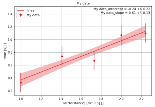
When plotting data and fitting them to a line (or other function), it is important to make sure that the values have at least an uncertainty in the quantity that is being plotted on the y axis. In this case, we have assumed that all of the measurements of time have an uncertainty of 0.15 s and that the measurements of the distance have no (or negligible) uncertainties.
Since we expect the slope of the data to be k, finding the line of best fit provides us a with method to determine k by using all of the data points. In this case, we find that k = (0.61 ± 0.13) \text{sm}^{−\frac{1}{2}}. Performing a linear fit of the data is the best way to determine a constant of proportionality between the measurements. Note that we expect the intercept to be equal to zero according to our model, but the best fit line has an intercept of (−0.24 ± 0.22) s, which is slightly below, but consistent, with zero. From these data, we would conclude that our measurements are consistent with Chloe’s Theory. Again, remember that we can never confirm a theory, we can only exclude it; in this case, we cannot exclude Chloe’s Theory.
Reporting measured values
Now that you know how to attribute an uncertainty to a measured quantity and then propagate that uncertainty to a derived quantity, you are ready to present your measurement to the world. In order to conduct “good science”, your measurements should be reproducible, clearly presented, and precisely described. Here are general rules to follow when reporting a measured number:
- Indicate the units, preferably SI units (use derived SI units, such as newtons, when appropriate).
- Include a description of how the uncertainty was determined (if it is a direct measurement, how did you choose the uncertainty? If it is a derived quantity, how did you propagate the uncertainty?).
- Show no more than 2 “significant digits”4 in the uncertainty and format the central value to the same decimal as the uncertainty.
- Use scientific notation when appropriate (usually numbers bigger than 1000 or smaller than 0.01).
- Factor out the power 10 from the central value and uncertainty (e.g. (10123 ± 310) m would be better presented as (10.12 ± 0.31) × 10^{3} m or (101.2 ± 3.1) × 10^{2} m).
Someone has measured the average height of tables in the laboratory to be 1.0535 m with a standard deviation of 0.0525 m. What is the best way to present this measurement?
- (1.0535 ± 0.0525) m
- (1.054 ± 0.053) m
- (105.4 ± 5.3) × 10^{−2} m
- (105.35 ± 5.25) cm
- Answer
Comparing model and measurement-discussing a result
In order to advance science, we make measurements and compare them to a theory or model prediction. We thus need a precise and consistent way to compare measurements with each other and with predictions. Suppose that we have measured a value for Chloe’s constant k = (0.44 ± 0.09)\text{sm}^{-\frac{1}{2}}. Of course, Chloe’s theory does not predict a value for k, only that fall time is proportional to the square root of the distance fallen. Isaac Newton’s Universal Theory of Gravity does predict a value for k of 0.45\text{sm}^{-\frac{1}{2}} with negligible uncertainty. In this case, since the model (theoretical) value easily falls within the range given by our uncertainty, we would say that our measurement is consistent (or compatible) with the theoretical prediction.
Suppose that, instead, we had measured k = (0.55 ± 0.08)\text{sm}^{-\frac{1}{2}} so that the lowest value compatible with our measurement, k = 0.55\text{sm}^{-\frac{1}{2}} − 0.08\text{sm}^{-\frac{1}{2}} = 0.47\text{sm}^{-\frac{1}{2}}, is not compatible with Newton’s prediction. Would we conclude that our measurement invalidates Newton’s theory? The answer is: it depends... What “it depends on” should always be discussed any time that you present a measurement (even if it happened that your measurement is compatible with a prediction - maybe that was a fluke). Below, we list a few common points that should be addressed when presenting a measurement that will guide you into deciding whether your measurement is consistent with a prediction:
- How was the uncertainty determined and/or propagated? Was this reasonable?
- Are there systematic effects that were not taken into account when determining the uncertainty? (e.g. reaction time, parallax, something difficult to reproduce).
- Are the relative uncertainties reasonable based on the precision that you would reasonable expect?
- What assumptions were made in calculating your measured value?
- What assumptions were made in determining the model prediction?
In the above, our value of k = (0.55 ± 0.08)\text{sm}^{-\frac{1}{2}} is the result of propagating the uncertainty in t which was found by using the standard deviation of the values of t. It is thus conceivable that the true value of t, and therefore of k, is outside the range that we quote. Since our value of k is still quite close to the theoretical value, we would not claim to have invalidated Newton’s theory with this measurement. Our uncertainty in k is σ_{k} = 0.08\text{sm}^{-\frac{1}{2}}, and the difference between our measured and the theoretical value is only 1.25σ_{k}, so very close to the value of the uncertainty.
In a similar way, we would discuss whether two different measurements, each with an uncertainty, are compatible. If the ranges given by uncertainties in two values overlap, then they are clearly consistent and compatible. If, on the other hand, the ranges do not overlap, they could be inconsistent or the discrepancy might instead be the result of how the uncertainties were determined and the measurements could still be considered consistent.