
7.2: Rotating Reference Frames


- Last updated
- Dec 30, 2020
- Save as PDF

( \newcommand{\kernel}{\mathrm{null}\,}\)
In Section 4.3, we considered what happens if we considered the (linear) motion of an object from a stationary (‘lab frame’) or co-moving point of view, with special attention for the center of mass frame. These frames were moving with constant velocity with respect to each other, and were all inertial frames - Newton’s first and second laws hold in all inertial frames. In this section, we’ll consider a rotating reference frame, where instead of co-moving with a linear velocity, we co-rotate with a constant angular velocity. Rotating reference frames are not inertial frames, as to keep something rotating (and thus change the direction of the linear velocity) requires the application of a net force. Instead, as we’ll see, in a rotating frame of reference we’ll get all sorts of fictitious forces - forces that have no real physical source, like gravity or electrostatics, but originate from the fact that we’re in a rotating reference frame.
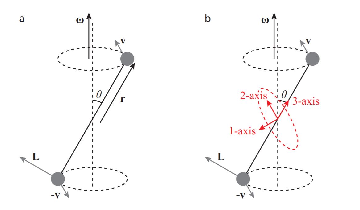
In a rotating reference frame, the direction of the basis vectors changes over time (as measured with respect to the stationary lab frame - this is different from the linearly co-moving frames, where the directions of the basis vectors remained constant). To see how the basis vectors change over time, we can simply calculate their linear velocity, using Equation 5.1.5:
dˆxdt=ω׈x,dˆydt=ω׈y,dˆzdt=ω׈z
We can now easily determine the change of an arbitrary vector u=uxˆx+uyˆy+uzˆz over time:
dudt=(∂ux∂tˆx+∂uy∂tˆy+∂uz∂tˆz)+(uxdˆxdt+uydˆydt+uzdˆzdt)=δuδt+ω×u
where δuδt is defined by Equation ???, and represents the time derivative of u in the rotating basis1. We see that in addition to the ‘regular’ time derivative, acting on the components of u, we get an additional term ω×u due to the rotation of the system. Note that for u=ω, we find that dωdt=δωδt=˙ω, i.e., the time derivative of the rotation vector is the same in the stationary and rotating frames.
The prime example of a vector is of course the position vector r of a particle, the second derivative of which appears in Newton’s second law of motion. We’ll calculate that second derivative for a position vector in a rotating coordinate frame. The first derivative is a simple application of Equation ???:
drdt=δrδt+ω×r
To get the second derivative, we apply ??? to the velocity vector found in ???:
d2rdt2=ddt(δrδt+ω×r)=δδt(δrδt+ω×r)+ω×(δrδt+ω×r)=δ2rδt2+δωδt×r+2ω×δrδt+ω×(ω×r)
Like in the two-dimensional case given by Equation 6.2.3, we find that the acceleration in a rotating reference frame picks up extra terms compared to a stationary (or more general, inertial) frame. To get a complete picture, we also allow the origin of the rotating frame to be different from that of the stationary lab frame. Let rlab be the position vector in the lab frame, R the vector pointing from the origin of the lab frame to that of the rotating frame, and r the position vector in the rotating frame. We then have rlab=R+r, and for the second derivative of rlab we find:
d2rlabdt2=d2rdt2+d2Rdt2=δ2rδt2+ω×(ω×r)+2ω×δrδt+δωδt×r+d2Rdt2
We can substitute Equation 7.2.6 in Newton’s second law of motion in the lab frame (i.e., just F=drlabdt) to find the expression for that law in the rotating frame:
mδ2rδt2=F−m[ω×(ω×r)+2ω×v+˙ω×r+d2Rdt2]
where we defined v=δrδt as the velocity in the rotating frame, and used that the time derivative of ω is the same in both the stationary and the rotating frame. We find that we get four correction terms to the force due to our transition to a rotating frame. They are not ‘real’ forces like gravity or friction, as they vanish in the lab frame, but you can easily experience their effects, when you’re in a turning car or rotating carousel. As they have no physical origin, we call these forces fictitious. They are known as the centrifugal, Coriolis, azimuthal, and translational force, respectively:
Fcf=−mω×(ω×r)
FCor=−2mω×v
Faz=−m˙ω×r
Ftrans=−md2Rdt2
We encountered the centrifugal, Coriolis and azimuthal force before in Section 6.2. To see how the expressions above connect to the planar versions, let us pick the coordinates of the rotating frame such that the direction of ω coincides with the z-axis. The rotational motion and the forces can then be described in terms of the cylindrical coordinates consisting of the polar coordinates (ρ,θ) in the xy-plane and z along the z-axis (note that we use ρ=√x2+y2 for the radial distance in the xy-plane instead of r, as r is now the distance from the origin to our point in three dimensions). For the centrifugal force we have ω⋅Fcf=0, so it lies in our newly defined xy-plane, and in cylindrical coordinates it can be expressed as
Fcf=−m[ω(ω⋅r)−ω2r]=mω2(xˆx+yˆy)=mω2ρˆρ
The centrifugal force is thus nothing but minus the centripetal force, which we already encountered for uniform rotational motion in Equation 5.2.1, and as the second term in 6.2.5. The centrifugal force is the force you ‘feel’ pushing you sidewards when your car makes a sharp turn, and is also responsible for creating the parabolic shape of the water surface in a spinning bucket, see Problem 7.4.
The Coriolis force is present whenever a particle is moving with respect to the rotating coordinates, and tends to deflect particles from a straight line (which you’d get in an inertial reference frame). We have ω⋅FCor = \boldsymbol{v} \cdot \boldsymbol{F}_{\mathrm{Cor}}\) = 0\), so the Coriolis force is perpendicular to both the rotation and velocity vectors - note that this is the velocity in the rotating frame. In the two-dimensional case, we had FmathrmCor=2m˙ρωˆθ (Equation 6.2.7), which for a velocity in the radial direction, ˙ρ, gives a force in the angular direction ˆθ.
The azimuthal force occurs when the rotation vector of our rotating system changes - i.e., when the rotation speeds up or decelerates, or the plane of rotation alters. In either case we have r⋅FCor=0, so the force is perpendicular to the position vector. If it is the magnitude of the rotation vector that changes, and we again take the rotation vector to lie along the z-axis in the rotating frame, ˙ω also lies along the z-axis, and we get
Faz=−m˙ωˆz×r=−mr¨θˆθ
so the azimuthal force is minus m times the tangential acceleration α (see Equation 5.1.8), or minus the first term of 6.2.6.
The translational force finally occurs when the rotating reference frame’s origin accelerates with respect to that of the stationary lab frame. You also feel it if the ‘rotating’ reference frame is actually not rotating, but only accelerating linearly - it’s the force that pushes you back in your seat when your car or train accelerates.
1 Some authors use the notation (dudt)rot for δuδt.