7.3: Rotations About an Arbitrary Axis

In Chapter 5, we studied the rotation of rigid bodies about an axis of symmetry. For these cases, we have $\boldsymbol{L} = I \boldsymbol{\omega}$, where I is the moment of inertia with respect to the rotation axis. We already noted that $I$ depends on which axis we pick, and that the proportional relation between the rotation vector and angular momentum is not the most general possibility. In this section, we’ll derive the more general form, in which the number I is replaced by a 2-tensor, i.e., a map from a vector space (here $\mathbb{R}^{3}$) into itself, represented by a 3×3 matrix.

Moment of Inertia Tensor

To arrive at the more general relation between $\boldsymbol{L}$ and $\boldsymbol{\omega}$, we go back to the original definition of $\boldsymbol{L} = \boldsymbol{r} \times \boldsymbol{p}$, and consider the motion of a dumbbell around an axis which is not a symmetry axis (see Figure 7.2.1). If the dumbbell makes an angle $\theta$ with the rotation axis, and rotates counter-clockwise as seen from the top, we get:

$$\begin{align} \boldsymbol{L} &=m \boldsymbol{r} \times \boldsymbol{v}+m(-\boldsymbol{r}) \times(-\boldsymbol{v}) \\[4pt] &=2 m \boldsymbol{r} \times(\boldsymbol{\omega} \times \boldsymbol{r}) \\[4pt] &=2 m[\boldsymbol{\omega}(\boldsymbol{r} \cdot \boldsymbol{r})-\boldsymbol{r}(\boldsymbol{r} \cdot \boldsymbol{\omega})] \\[4pt] &=2 m r^{2} \boldsymbol{\omega}-2 m \omega r \cos \theta \boldsymbol{r} \label{angularmomentum} \end{align}$$

where we used Equation 5.1.5 relating the linear velocity $\boldsymbol{v}$ to the rotational velocity $\boldsymbol{\omega}$ through $\boldsymbol{v} = \boldsymbol{\omega} \times \boldsymbol{r}$. Equation $\ref{angularmomentum}$ shows that for a rotation about an arbitrary axis through the center of the dumbbell, we get two terms in $\boldsymbol{L}$. The first term, $2mr^2 \boldsymbol{\omega}$, is the rotation about an axis perpendicular to the dumbbell, and equals $I \boldsymbol{\omega}$ for $I = 2mr^2$, as we found in Section 5.4. The second term, ($−2m \omega r \cos{\theta} \boldsymbol{r}$), tells us that in general we also get a component of $\boldsymbol{L}$ along the axis pointing from the rotation center to the rotating mass (i.e., the arm). Note that the two terms cancel when $\theta = \pi /2$, as we’d expect for in that case the moment of inertia of the dumbbell is zero.

We can easily generalize Equation $\ref{angularmomentum}$ to any set of masses $m_{\alpha}$ with position vectors $\boldsymbol{r}_{\alpha}$ (where the index $\alpha$ runs over all particles), and with a rotation $\boldsymbol{\omega}$ about an arbitrary axis:

$$\boldsymbol{L}=\sum_{\alpha} m_{\alpha} \boldsymbol{r}_{\alpha} \times\left(\boldsymbol{\omega} \times \boldsymbol{r}_{\alpha}\right) \equiv \boldsymbol{I} \cdot \boldsymbol{\omega} \label{moitensor}$$

The moment of inertia tensor is defined by Equation $\ref{moitensor}$. It is a symmetric tensor, mapping a vector $\boldsymbol{\omega}$ in $\mathbb{R}^{3}$ onto another vector $\boldsymbol{L}$ in $\mathbb{R}^{3}$. In Cartesian coordinates, we can express its nine components as three moments of inertia about the x, y and z axes, which will be the diagonal terms of $\boldsymbol{I}$:

$$I_{x x}=\sum_{\alpha} m_{\alpha}\left(y_{\alpha}^{2}+z_{\alpha}^{2}\right) \quad I_{y y}=\sum_{\alpha} m_{\alpha}\left(x_{\alpha}^{2}+z_{\alpha}^{2}\right) \quad I_{z z}=\sum_{\alpha} m_{\alpha}\left(x_{\alpha}^{2}+y_{\alpha}^{2}\right) \label{momsofinert}$$

and three products of inertia for the off-diagonal components:

$$I_{x y}=I_{y x}=-\sum_{\alpha} m_{\alpha} x_{\alpha} y_{\alpha} \quad I_{x z}=I_{z x}=-\sum_{\alpha} m_{\alpha} x_{\alpha} z_{\alpha} \quad I_{y z}=I_{z y}=-\sum_{\alpha} m_{\alpha} y_{\alpha} z_{\alpha} \label{prodsofinert}$$

We can also write Equations $\ref{momsofinert}$ and $\ref{prodsofinert}$ more succinctly using index notation, where $i$ and $j$ run over $x, y$ and $z$, and we use the Kronecker delta $\delta_{ij}$ which is one if $i = j$ and zero if $i \neq j$:

$$I_{i j}=\sum_{\alpha} m_{\alpha}\left(r^{2} \delta_{i j}-r_{i} r_{j}\right)$$

Equations $\ref{momsofinert}$ and $\ref{prodsofinert}$ generalize to continuous objects in the same way Equation 5.4.2 generalized to 5.4.3. Using the index notation again, we can explicitly write:

$$I_{i j}=\int_{V}\left(r^{2} \delta_{i j}-r_{i} r_{j}\right) \rho(\boldsymbol{r}) \mathrm{d} V$$

The moment of inertia tensor contains all information about the rotational inertia of an object (or a collection of particles) about any axis. In particular, if one of the axes (say the z-axis) is an axis of symmetry, we get that $I_{xz} = I_{yz} = 0$, and for rotations about that axis (so $\boldsymbol{\omega} = \omega \boldsymbol{\hat{z}}$), we retrieve $\boldsymbol{L} = I_z \boldsymbol{\omega}$.

In addition to calculating the angular momentum, we can also use the moment of inertia tensor for calculating the kinetic energy for rotations about an arbitrary axis. We have:

$$\begin{aligned} K &=\frac{1}{2} \sum_{\alpha} m_{\alpha} \boldsymbol{v}_{\alpha} \cdot \boldsymbol{v}_{\alpha} \\ &=\frac{1}{2} \sum_{\alpha} m_{\alpha}\left(\boldsymbol{\omega} \times \boldsymbol{r}_{\alpha}\right) \cdot\left(\boldsymbol{\omega} \times \boldsymbol{r}_{\alpha}\right) \\ &=\frac{1}{2} \boldsymbol{\omega} \cdot\left[\sum_{\alpha} m_{\alpha} \boldsymbol{r}_{\alpha} \times\left(\boldsymbol{\omega} \times \boldsymbol{r}_{\alpha}\right)\right] \\ &=\frac{1}{2} \boldsymbol{\omega} \cdot \boldsymbol{L}=\frac{1}{2} \boldsymbol{\omega} \cdot \boldsymbol{I} \cdot \boldsymbol{\omega} \end{aligned}$$

Euler's Equations

In the lab frame, we have Equation 5.7.1 relating the torque and the angular momentum. We used this equation to prove conservation of angular momentum in the absence of a net external torque, and to study precession. However, for rotations about an arbitrary axis, it is easier to transform to a frame in which we rotate with the object, much like moving with the center of mass makes the study of collisions much easier. We’ve already done the math for transforming to a co-rotating frame in Section 7.2; here we only need the result in Equation 7.2.2 to find the time derivative of the angular momentum in the rotating frame. Equation 5.7.1 then translates to:

$$\begin{align} \boldsymbol{\tau} &=\frac{\delta \boldsymbol{L}}{\delta t}+\boldsymbol{\omega} \times \boldsymbol{L} \\[4pt] &=\boldsymbol{I} \cdot \dot{\boldsymbol{\omega}}+\boldsymbol{\omega} \times(\boldsymbol{I} \cdot \boldsymbol{\omega}) \label{tau} \end{align}$$

Now since $\boldsymbol{I}$ is symmetric, all its eigenvalues are real, and its eigenvectors are a basis for $\mathbb{R}^{3}$; moreover, for distinct eigenvalues the eigenvectors are orthogonal, so from the eigenvector basis we can easily construct an orthonormal basis $\left(\hat{\boldsymbol{e}}_{1}, \hat{\boldsymbol{e}}_{2}, \hat{\boldsymbol{e}}_{3}\right)$ of eigenvectors corresponding to the three eigenvalues $I_{1}, I_{2}$ and $I_{3}$. If we express the moment of inertia tensor in this orthonormal eigenvector basis, its representation becomes a simple diagonal matrix, $\boldsymbol{I}=\operatorname{diag}\left(I_{1}, I_{2}, I_{3}\right)$. We call the directions $\hat{\boldsymbol{e}}_{i}$ the principal axes of our rotating object, and the associated eigenvalues the principal moments of inertia. The construction of the principal axes and moments of inertia works for any object - including ones that do not exhibit any kind of symmetry. If an object does have a symmetry axis, that axis is usually also a principal axis, as can easily be checked by calculating the products of inertia with respect to that axis (they vanish for a principal axis).

Leonhard Euler

Leonhard Euler (1707-1783) was a Swiss mathematician who made major contributions to many different branches of mathematics, and, by application, physics. He also introduced much of the modern mathematical terminology and notation, including the concept of (mathematical) functions. Euler was possibly the most prolific mathematician who ever lived, and likely is the person with the most equations and formula’s named after him. Although his father, who was a pastor, encouraged Euler to follow in his footsteps, Euler’s tutor, famous mathematician (and family friend) Johann Bernoulli convinced both father and son that Euler’s talent for mathematics would make him a giant in the field. Famous examples of Euler’s work include his contributions to graph theory (the Köningsberg bridges problem), the relation $e^{i \pi} +1 = 0$ between five fundamental mathematical numbers named after him, his work on power series, a method for numerically solving differential equations, and his work on fluid mechanics (in which there is also an ‘Euler’s equation’).

Figure $\PageIndex{1}$: Portrait of Leonhard Euler by Jakob Handmann (1753) [22].

If we express our rotational quantities in the principal axis basis $\left\{\text {unitvece}_{i}\right\}$ of our rotating object, our equations become much simpler. We have

$$\boldsymbol{L}=\boldsymbol{I} \cdot \boldsymbol{\omega}=\left(\begin{array}{ccc}{I_{1}} & {0} & {0} \\ {0} & {I_{2}} & {0} \\ {0} & {0} & {I_{3}}\end{array}\right)\left(\begin{array}{c}{\omega_{1}} \\ {\omega_{2}} \\ {\omega_{3}}\end{array}\right)=\left(\begin{array}{c}{I_{1} \omega_{1}} \\ {I_{2} \omega_{2}} \\ {I_{3} \omega_{3}}\end{array}\right)$$

or in components: $L_{i}=I_{i} \omega_{i}$. Equation $\ref{tau}$ simplifies to:

$$\boldsymbol{\tau}=\left(\begin{array}{c}{I_{1} \dot{\omega}_{1}} \\ {I_{2} \dot{\omega}_{2}} \\ {I_{3} \dot{\omega}_{3}}\end{array}\right)+\left(\begin{array}{c}{\omega_{1}} \\ {\omega_{2}} \\ {\omega_{3}}\end{array}\right) \times\left(\begin{array}{c}{I_{1} \omega_{1}} \\ {I_{2} \omega_{2}} \\ {I_{3} \omega_{3}}\end{array}\right)$$

which gives for the three components of the torque:

$$\begin{array}{l}{\tau_{1}=I_{1} \dot{\omega}_{1}+\left(I_{3}-I_{2}\right) \omega_{3} \omega_{2}} \\ {\tau_{2}=I_{2} \dot{\omega}_{2}+\left(I_{1}-I_{3}\right) \omega_{1} \omega_{3}} \\ {\tau_{3}=I_{3} \dot{\omega}_{3}+\left(I_{2}-I_{1}\right) \omega_{2} \omega_{1}} \label{t1t2t3} \end{array}$$

Equations $\ref{t1t2t3}$ are known as Euler’s equations (of a rotating object - the classification is necessary as there are many equations associated with Euler).

As an example, let’s apply Euler’s equations to our dumbbell. We take the origin at the pivot, i.e., where the rotation axis crosses the dumbbell’s own axis. The dumbbell does have rotational symmetry, about the axis connecting the two masses - let’s call that the 3-axis. The other two axes then span the plane perpendicular to the dumbbell; we can pick any orthonormal pair for the 1 and 2-axes. The rotation vector in this basis is given by

$$\boldsymbol{\omega}=\left(\begin{array}{c}{\omega_{1}} \\ {\omega_{2}} \\ {\omega_{3}}\end{array}\right)=\omega\left(\begin{array}{c}{0} \\ {\sin \theta} \\ {\cos \theta}\end{array}\right)$$

The products of inertia vanish; the principal moments are given by $I_{1}=I_{2}=\frac{1}{2} m d^{2}$ (with $d$ the distance between the two masses) and $I_3 = 0$. As long as the rotational velocity is constant ($\dot{\boldsymbol{\omega}}=0$), we get from Euler’s equations that $\tau_{2}=\tau_{3}=0$, and $\tau_{1}=-\frac{1}{2} m d^{2} \omega^{2} \sin \theta \cos \theta$. We can thus rotate our dumbbell about an axis that’s not a symmetry axis, but at a price: it exerts a torque on its support, which in turn exerts a countertorque to keep the dumbbell’s rotation axis in place. This torque will change the angular momentum of our dumbbell over time. If we remove the force exerting the counter-torque (e.g., if our dumbbell is supported at the pivot, remove the support), the dumbbell will turn, in our example about axis 2, until the rotation vector $\boldsymbol{\omega}$ has become parallel with the angular momentum vector $\boldsymbol{L}$.

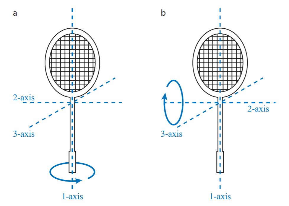
For the dumbbell, as it has a rotational symmetry, two of the principal moments are identical. There are many objects that have no such symmetry, but they still have three well-defined principal axes. While for the dumbbell rotation about any of the principal axes is stable, this is not the case for an object with three different principal moments. A good example is a tennis racket, whose principal axes are sketched in Figure 7.3.1. The accompanying theorem about the stability of rotations about these axes is easily demonstrated with a tennis racket, and bears its name.

Theorem $\PageIndex{1}$: Tennis Racket Theorem

If the three principal moments of inertia of an object are different (say $I_{1}<I_{2}<I_{3}$), then rotations about the principal axes 1 and 3 associated with the maximum and minimum moments $I_1$ and $I_3$ are stable, but those about the principal axis 2 associated with the intermediate moment $I_2$ are unstable.

Proof

For rotations about a principal axis, the torque is zero (by construction), so Euler’s equations read

$$\begin{array}{l}{\dot{\omega}_{1}+\frac{I_{3}-I_{2}}{I_{1}} \omega_{3} \omega_{2}=0} \\ {\dot{\omega}_{2}+\frac{I_{1}-I_{3}}{I_{2}} \omega_{1} \omega_{3}=0} \\ {\dot{\omega}_{3}+\frac{I_{2}-I_{1}}{I_{3}} \omega_{2} \omega_{1}=0}\end{array} \ref{eulers}$$

If we rotate about axis 1, then $\omega _2$ and $\omega _3$ are (at least initially) very small, so the first line in $\ref{eulers}$ gives $\dot{\omega}_{1}=0$. We can then derive an equation for $\omega _2$ by taking the time derivative of the second line of $\ref{eulers}$ and using the third line for $\dot{\omega}_{3}$, which gives:

$$0=\ddot{\omega}_{2}+\frac{I_{1}-I_{3}}{I_{2}}\left(\dot{\omega}_{1} \omega_{3}+\omega_{1} \omega_{3}\right)=\ddot{\omega}_{2}-\frac{I_{1}-I_{3}}{I_{2}} \frac{I_{2}-I_{1}}{I_{3}} \omega_{1}^{2} \omega_{2}$$

Now $\frac{\left(I_{1}-I_{3}\right)}{I_{2}}<0, \frac{\left(I_{2}-I_{1}\right)}{I_{3}}>0$, and $\omega_{1}^{2}>0$, and $\omega _2$ satisfies the differential equation $\ddot{\omega}_{2}=-c \omega_{2}$, with $c > 0$. Solutions to this equation are of course sines and cosines with constant amplitude. Although $\omega _2$ can thus be finite, its amplitude does not grow over time (and will in fact decrease due to drag), so rotations about axis 2 are opposed. Similarly, we find that rotations about axis 3 cannot grow in amplitude either, and rotations about axis 1 are stable. We can repeat the same argument for axes 2 and 3. For axis 3, we find that rotations about the other two axes are likewise opposed, so rotations about this axis are stable as well. For axis 2 on the other hand, we find that

$$0=\ddot{\omega}_{1}-\frac{I_{3}-I_{2}}{I_{1}} \frac{I_{2}-I_{1}}{I_{3}} \omega_{2}^{2} \omega_{1}$$

or $\ddot{\omega}_{1}=c \omega_{1}$, with $c$ another positive constant. Solutions to this equation are not sines and cosines, but exponential: $\omega_{1}(t)=A \exp (\sqrt{c} t)+B \exp (-\sqrt{c} t)$, which means that for any finite initial rotation about the 1 axis, the amplitude of this rotation will grow over time, and rotations about the 2-axis are thus unstable.

Figure $\PageIndex{2}$: The three principal axes of a tennis racket.