
2.2: Acceleration


- Last updated
- Nov 5, 2020
- Save as PDF

( \newcommand{\kernel}{\mathrm{null}\,}\)
Average and Instantaneous Acceleration
Just as we defined average velocity in the previous chapter, using the concept of displacement (or change in position) over a time interval Δt, we define average acceleration over the time Δt using the change in velocity:
aav=ΔvΔt=vf−vitf−ti.
Here, vi and vf are the initial and final velocities, respectively, that is to say, the velocities at the beginning and the end of the time interval Δt. As was the case with the average velocity, though, the average acceleration is a concept of somewhat limited usefulness, so we might as well proceed straight away to the definition of the instantaneous acceleration (or just “the” acceleration, without modifiers), through the same sort of limiting process by which we defined the instantaneous velocity:
a=limΔt→0ΔvΔt.
Everything that we said in the previous chapter about the relationship between velocity and position can now be said about the relationship between acceleration and velocity. For instance (if you know calculus), the acceleration as a function of time is the derivative of the velocity as a function of time, which makes it the second derivative of the position function:
a=dvdt=d2xdt2
(and if you do not know calculus yet, do not worry about the superscripts “2” on that last expression! It is just a weird notation that you will learn someday.)
Similarly, we can “read off” the instantaneous acceleration from a velocity versus time graph, by looking at the slope of the line tangent to the curve at any point. However, if what we are given is a position versus time graph, the connection to the acceleration is more indirect. Figure 2.2.1 provides you with such an example. See if you can guess at what points along this curve the acceleration is positive, negative, or zero.
The way to do this “from scratch,” as it were, is to try to figure out what the velocity is doing, first, and infer the acceleration from that. Here is how that would go:
Starting at t = 0, and keeping an eye on the slope of the x-vs-t curve, we can see that the velocity starts at zero or near zero and increases steadily for a while, until t is a little bit more than 2 s (let us say, t = 2.2 s for definiteness). That would correspond to a period of positive acceleration, since Δv would be positive for every Δt in that range.
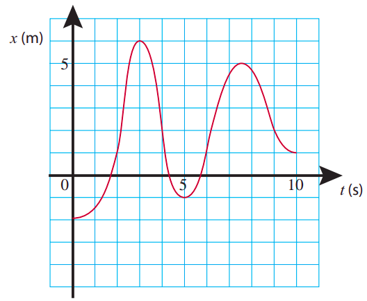
Between t = 2.2 s and t = 2.5 s, as the object moves from x = 2 m to x = 4 m, the velocity does not appear to change very much, and the acceleration would correspondingly be zero or near zero. Then, around t = 2.5 s, the velocity starts to decrease noticeably, becoming (instantaneously) zero at t =3 s (x = 6 m). That would correspond to a negative acceleration. Note, however, that the velocity afterwards continues to decrease, becoming more and more negative until around t = 4 s. This also corresponds to a negative acceleration: even though the object is speeding up, it is speeding up in the negative direction, so Δv, and hence a, is negative for every time interval there. We conclude that a<0 for all times between t = 2.5 s and t = 4 s.
Next, as we just look past t = 4 s, something else interesting happens: the object is still going in the negative direction (negative velocity), but now it is slowing down. Mathematically, that corresponds to a positive acceleration, since the algebraic value of the velocity is in fact increasing (a number like −3 is larger than a number like −5). Another way to think about it is that, if we have less and less of a negative thing, our overall trend is positive. So the acceleration is positive all the way from t = 4 s through t = 5 s (where the velocity is instantaneously zero as the object’s direction of motion reverses), and beyond, until about t = 6 s, since between t = 5 s and t = 6 s the velocity is positive and growing.
You can probably figure out on your own now what happens after t = 6 s, reasoning as I did above, but you may also have noticed a pattern that makes this kind of analysis a lot easier. The acceleration (as those with a knowledge of calculus may have understood already), being proportional to the second derivative of the function x(t) with respect to t, is directly related to the curvature of the x-vs-t graph. As figure 2.2.2 below shows, if the graph is concave (sometimes called “concave upwards”), the acceleration is positive, whereas it is negative whenever the graph is convex (or “concave downwards”). It is (instantly) zero at those points where the curvature changes (which you may know as inflection points), as well as over stretches of time when the x-vs-t graph is a straight line (motion with constant velocity).
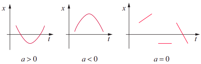
Figure 2.2.3 shows position, velocity, and acceleration versus time for a hypothetical motion case. Please study it carefully until every feature of every graph makes sense, relative to the other two! You will see many other examples of this in the homework and the lab.
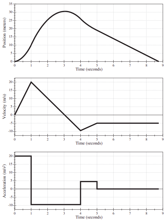
Notice that, in all these figures, the sign of x or v at any given time has nothing to do with the sign of a at that same time. It is true that, for instance, a negative a, if sustained for a sufficiently long time, will eventually result in a negative v (as happens, for instance, in Figure 2.2.3 over the interval from t = 1 to t = 4 s) but this may take a long time, depending on the size of a and the initial value of v. The graphical clues to follow, instead, are: the acceleration is given by the slope of the tangent to the v-vs-t curve, or the curvature of the x-vs-t curve, as explained in Figure 2.2.2; and the velocity is given by the slope of the tangent to the x-vs-t curve.
(Note: To make the interpretation of Figure 2.2.3 simpler, I have chosen the acceleration to be “piecewise constant,” that is to say, constant over extended time intervals and changing in value discontinuously from one interval to the next. This is physically unrealistic: in any real-life situation, the acceleration would be expected to change more or less smoothly from instant to instant. We will see examples of that later on, when we start looking at realistic models of collisions.)
Motion With Constant Acceleration
A particular kind of motion that is both relatively simple and very important in practice is motion with constant acceleration (see Figure 2.2.3 again for examples). If a is constant, it means that the velocity changes with time at a constant rate, by a fixed number of m/s each second. (These are, incidentally, the units of acceleration: meters per second per second, or m/s2.) The change in velocity over a time interval Δt is then given by
which can also be written
v=vi+a(t−ti).
Equation (???) is the form of the velocity function (v as a function of t) for motion with constant acceleration. This, in turn, has to be the derivative with respect to time of the corresponding position function. If you know simple derivatives, then, you can verify that the appropriate form of the position function must be
or in terms of intervals,
Most often Equation (???) is written with the implicit assumption that the initial value of t is zero:
x=xi+vit+12at2.
This is simpler, but not as general as Equation (???). Always make sure that you know what conditions apply for any equation you decide to use!
As you can see from Equation (???), for intervals during which the acceleration is constant, the velocity vs. time curve should be a straight line. Figure 2.2.3 illustrates this. Equation (???), on the other hand, shows that for those same intervals the position vs. time curve should be a (portion of a) parabola, and again this can be seen in Figure 2.2.3 (sometimes, if the acceleration is small, the curvature of the graph may be hard to see; this happens in Figure 2.2.3 for the interval between t = 4 s and t = 5 s).
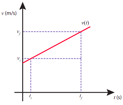
The observation that v-vs-t is a straight line when the acceleration is constant provides us with a simple way to derive Equation (???), when combined with the result (from the end of the previous chapter) that the displacement over a time interval Δt equals the area under the v-vs-t curve for that time interval. Indeed, consider the situation shown in Figure 2.2.4. The total area under the segment shown is equal to the area of a rectangle of base Δt and height vi, plus the area of a triangle of base Δt and height vf−vi. Since vf−vi=aΔt, simple geometry immediately yields Equation (???), or its equivalent (???).
Lastly, consider what happens if we solve Equation (???) for Δt and substitute the result in (???). We get
Δx=viΔva+(Δv)22a.
Letting Δv=vf−vi, a little algebra yields
This is a handy little result that can also be seen to follow, more directly, from the work-energy theorems to be introduced in Chapter 71.
1 In fact, equation (???) turns out to be so handy that you will probably find yourself using it over and over this semester, and you may even be tempted to use it for problems involving motion in two dimensions. However, unless you really know what you are doing, you should resist the temptation, since it is very easy to use Equation (???) incorrectly when the acceleration and the displacement do not lie along the same line. You should use the appropriate form of a work-energy theorem instead.
Acceleration as a Vector
In two (or more) dimensions we introduce the average acceleration vector
→aav=Δ→vΔt=1Δt(→vf−→vi)
whose components are aav,x=Δvx/Δt, etc.. The instantaneous acceleration is then the vector given by the limit of Equation (???) as Δt→0, and its components are, therefore, ax=dvx/dt,ay=dvy/dt, . . .
Note that, since →vi and →vf in Equation (???) are vectors, and have to be subtracted as such, the acceleration vector will be nonzero whenever →vi and →vf are different, even if, for instance, their magnitudes (which are equal to the object’s speed) are the same. In other words, you have accelerated motion whenever the direction of motion changes, even if the speed does not.
As long as we are working in one dimension, I will follow the same convention for the acceleration as the one I introduced for the velocity in Chapter 1: namely, I will use the symbol a, without a subscript, to refer to the relevant component of the acceleration (ax,ay,...), and not to the magnitude of the vector →a.
Acceleration in Different Reference Frames
In Chapter 1 you saw that the following relation holds between the velocities of a particle P measured in two different reference frames, A and B:
→vAP=→vAB+→vBP.
What about the acceleration? An equation like (???) will hold for the initial and final velocities, and subtracting them we will get
Δ→vAP=Δ→vAB+Δ→vBP.
Now suppose that reference frame B moves with constant velocity relative to frame A. In that case, →vAB,f=→vAB,i, so Δ→vAB = 0, and then, dividing Equation (???) by Δt, and taking the limit Δt→0, we get
→aAP=→aBP (for constant →vAB).
So, if two reference frames are moving at constant velocity relative to each other, observers in both frames measure the same acceleration for any object they might both be tracking.
The result Equation (???) means, in particular, that if we have an inertial frame then any frame moving at constant velocity relative to it will be inertial too, since the respective observers’ measurements will agree that an object’s velocity does not change (otherwise put, its acceleration is zero) when no forces act on it. Conversely, an accelerated frame will not be an inertial frame, because Equation (???) will not hold. This is consistent with the examples I mentioned in Section 2.1 (the bouncing plane, the car coming to a stop). Another example of a non-inertial frame would be a car going around a curve, even if it is going at constant speed, since, as I just pointed out above, this is also an accelerated system. This is confirmed by the fact that objects in such a car tend to move—relative to the car—towards the outside of the curve, even though no actual force is acting on them.