8.4: Coupled Oscillators

Two Coupled Pendulums

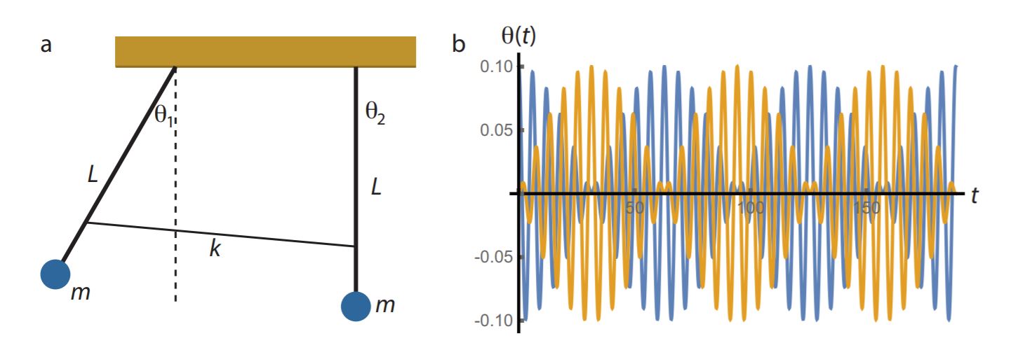
A beautiful demonstration of how energy can be transferred from one oscillator to another is provided by two weakly coupled pendulums. Imagine we have two identical pendulums of length $L$ and mass $m$, which are connected by a weak spring with spring constant k (Figure $\PageIndex{1a}$).

Figure $\PageIndex{1}$: Motion of two coupled pendulums. (a) Sketch of the setup. Two identical pendulums of length $L$ and mass $m$ are connected through a weak spring of spring constant $k$. As our initial condition, we choose both pendulums at rest, with the right one in its equilibrium position and the left one given a finite amplitude. (b) Resulting motion of the two pendulums: left (blue) and right (orange).

The equation of motion of the combined system is then given by:

$$\begin{align} \dot{L} \ddot{\theta}_{1} &=-g \sin \theta_{1}-k L\left(\sin \theta_{1}-\sin \theta_{2}\right) \label{eqofmot1} \\ L \ddot{\theta}_{2} &=-g \sin \theta_{2}+k L\left(\sin \theta_{1}-\sin \theta_{2}\right) \label{eqofmot2} \end{align}$$

We will once again use the small angle expansion in which we can approximate $\sin \theta \approx \theta$, and identify $\omega_0 = \sqrt{\frac{g}{L}}$ as the frequency of each of the (uncoupled) pendulums. Equations $\ref{eqofmot1}$ and $\ref{eqofmot2}$ then become

$$\begin{align} \ddot{\theta}_1 &=-\omega_{0}^{2} \theta_{1}-k \theta_{1}+k \theta_{2} \label{ddottheta1} \\[4pt] \ddot{\theta}_2 &=-\omega_{0}^{2} \theta_{2}+k \theta_{1}-k \theta_{2} \label{ddottheta2} \end{align}$$

We can solve the system of coupled differential equations in Equations $\ref{ddottheta1}$ and $\ref{ddottheta2}$ easily by introducing two new variables: $\alpha=\theta_{1}+\theta_{2}$ and $\beta=\theta_{1}-\theta_{2}$, which gives us two uncoupled equations:

$$\begin{align} \ddot{\alpha} &=-\omega_{0}^{2} \alpha \label{ddotalpha} \\[4pt] \ddot{\beta} &=-\omega_{0}^{2} \beta-2 k \beta=-\left(\omega^{\prime}\right)^{2} \beta \label{ddotbeta} \end{align}$$

where $\left(\omega^{\prime}\right)^{2}=\omega_{0}^{2}+2 k$ or $\omega^{\prime}=\sqrt{2 k+g / L}$. Since Equations $\ref{ddotalpha}$ and $\ref{ddotbeta}$ are simply the equations of harmonic oscillators, we can write down their solutions immediately:

$$\begin{align} \alpha(t) &=A \cos \left(\omega_{0} t+\phi_{0}\right) \\ \beta(t) &=B \cos \left(\omega^{\prime} t+\phi^{\prime}\right) \end{align}$$

Converting back to the original variables $\theta _1$ and $\theta _2$ is also straightforward, and gives

$$\begin{align}{\theta_{1}=\frac{1}{2}(\alpha+\beta)=\frac{A}{2} \cos \left(\omega_{0} t+\phi_{0}\right)+\frac{B}{2} \cos \left(\omega^{\prime} t+\phi^{\prime}\right)} \\ {\theta_{2}=\frac{1}{2}(\alpha-\beta)=\frac{A}{2} \cos \left(\omega_{0} t+\phi_{0}\right)-\frac{B}{2} \cos \left(\omega^{\prime} t+\phi^{\prime}\right)}\end{align}$$

Let’s put in some specific initial conditions: we leave pendulum number 2 at rest in its equilibrium position $(\theta_{2}(0)=\dot{\theta}_{2}(0)=0)$ and give pendulum number 1 a finite amplitude but also release it at rest $(\theta_{1}(0)=\theta_{0}, \dot{\theta}_{1}(0)=0)$. Working out the four unknowns ($A, B, \phi_0$ and $\phi '$) is straightforward, and we get:

$$\begin{align}{\theta_{1}=\frac{\theta_{0}}{2} \cos \left(\omega_{0} t\right)+\frac{\theta_{0}}{2} \cos \left(\omega^{\prime} t\right)=\theta_{0} \cos \left(\frac{\omega_{0}+\omega^{\prime}}{2} t\right) \cos \left(\frac{\omega_{0}-\omega^{\prime}}{2} t\right)} \label{theta1} \\ {\theta_{2}=\frac{\theta_{0}}{2} \cos \left(\omega_{0} t\right)-\frac{\theta_{0}}{2} \cos \left(\omega^{\prime} t\right)=\theta_{0} \sin \left(\frac{\omega_{0}+\omega^{\prime}}{2} t\right) \sin \left(\frac{\omega^{\prime}-\omega_{0}}{2} t\right)} \label{theta2} \end{align}$$

The solution given by Equations $\ref{theta1}$ and $\ref{theta2}$ is plotted in Figure $\PageIndex{1}$. Note that the solutions have two frequencies (known as the eigenfrequencies of the system). The fast one, $\frac{1}{2}\left(\omega_{0}+\omega^{\prime}\right)$, which for a weak coupling constant $k$ is very close to the eigenfrequency $\omega_0$ of a single pendulum, is the frequency at which the pendulums oscillate. The do so in anti-phase, as expressed mathematically by the fact that one oscillation has a sine and the other a cosine (which is of course just a sine shifted over $\frac{\pi}{2}$). The second frequency, $\frac{1}{2}\left(\omega^{\prime}-\omega_{0}\right)$ is much slower, and represents the frequency at which the two pendulums transfer energy to each other, through the spring that couples them. In Figure $\PageIndex{1b}$, it is the frequency of the envelope of the amplitude of the oscillation of either of the pendulums. All these phenomena will return in the next section, in the study of waves, which travel in a medium in which many oscillators are coupled to one another (Figure $\PageIndex{2}$).

Figure $\PageIndex{2}$: Two pendula hanging from a string is an example of a pair of coupled oscillators. Notice the amplitude shift from one pendulum to the other in time (Public Domain; Lucas V. Barbosa via Wikipedia)

Normal Modes

For a system with only two oscillators, the technique we used above for solving the system of coupled Equations $\ref{eqofmot1}$ and $\ref{eqofmot2}$ is straightforward. It does however not generalize easily to systems with many oscillators. Instead, we can exploit the fact that the equations are linear and use techniques from linear algebra (as you may have guessed from the term eigenfrequency). We can rewrite Equations $\ref{eqofmot1}$ and $\ref{eqofmot2}$ in matrix form:

$$\frac{\mathrm{d}^{2}}{\mathrm{d} t^{2}}\left(\begin{array}{l}{\theta_{1}} \\ {\theta_{2}}\end{array}\right)=\left(\begin{array}{cc}{-\left(\omega_{0}^{2}+k\right)} & {k} \\ {k} & {-\left(\omega_{0}^{2}+k\right)}\end{array}\right)\left(\begin{array}{l}{\theta_{1}} \\ {\theta_{2}}\end{array}\right) \label{2oscmat}$$

Equation $\ref{2oscmat}$ is a homogeneous, second-order differential equation with constant coefficients, strongly resembling the equation for a simple, one-dimensional harmonic oscillator. Consequently, we may expect the solutions to look similar as well, so we try our usual Ansatz:

$$\left(\begin{array}{l}{\theta_{1}} \\ {\theta_{2}}\end{array}\right)=\left(\begin{array}{l}{C_{1}} \\ {C_{2}}\end{array}\right) e^{i \omega t} \label{ansatz}$$

where $C_1$ and $C_2$ are constants. Substituting $\ref{ansatz}$ in $\ref{2oscmat}$ gives

$$\left(\begin{array}{cc}{\omega_{0}^{2}+k} & {-k} \\ {-k} & {\omega_{0}^{2}+k}\end{array}\right)\left(\begin{array}{c}{C_{1}} \\ {C_{2}}\end{array}\right)=\omega^{2}\left(\begin{array}{c}{C_{1}} \\ {C_{2}}\end{array}\right) \label{subrslt}$$

which you hopefully recognize as an eigenvalue problem. Solving for the eigenvalues $\omega ^2$ gives:

$$\left(-\omega^{2}+\omega_{0}^{2}+k\right)^{2}-k^{2}=0 \label{eigenval}$$

The solutions of Equation $\ref{eigenval}$ unsurprisingly reproduce the frequencies of the uncoupled equations in Section 8.4.1:

$$\omega_{+}^{2}=\omega_{0}^{2}, \quad \omega_{-}^{2}=\omega_{0}^{2}+2 k.$$

The eigenvectors of $\ref{subrslt}$ are given by

$$\boldsymbol{C}_{+}=\frac{1}{\sqrt{2}}\left(\begin{array}{l}{1} \\ {1}\end{array}\right) \quad \text { for } \quad \omega_{+} \quad \text { and } \quad \mathbf{C}_{-}=\frac{1}{\sqrt{2}}\left(\begin{array}{c}{1} \\ {-1}\end{array}\right) \quad \text { for } \quad \omega_{-}$$

Note that the eigenvectors are orthogonal; this is a general property of the eigenvectors of symmetric matrices. Each eigenvector corresponds to a possible steady-state of motion of the system; these states are known as the normal modes (‘normal’ referring to the orthogonality of the eigenvectors). We can now immediately write down the most general solution of Equation $\ref{2oscmat}$ as a linear combination of the eigenmodes:

$$\left(\begin{array}{c}{\theta_{1}(t)} \\ {\theta_{2}(t)}\end{array}\right)=\frac{A_{+}}{2} e^{i\left(\omega_{+} t+\phi_{+}\right)}\left(\begin{array}{c}{1} \\ {1}\end{array}\right)+\frac{A_{-}}{2} e^{i\left(\omega_{-} t+\phi_{-}\right)}\left(\begin{array}{c}{1} \\ {-1}\end{array}\right)$$

where the amplitudes $A_{\pm}$ and phases $\phi_{\pm}$ are determined by the initial conditions.

Writing our system of equations in matrix form allows us to easily generalize both to asymmetric configurations (see Problem 8.7) and to systems with many coupled oscillators. An important example of the latter case is the study of vibrations in solids. Atoms or ions in solids typically form a crystal lattice, that can be modeled as a large number of masses coupled by springs. Such crystals can have complicated vibrational properties, that can be analyzed in terms of its normal modes. In particular the modes with a low energy can typically be accessed easily. They are known as phonons, and correspond to sound waves in the solid.