
11A: Relative Velocity
- Page ID
- 2467

\( \newcommand{\vecs}[1]{\overset { \scriptstyle \rightharpoonup} {\mathbf{#1}} } \)
\( \newcommand{\vecd}[1]{\overset{-\!-\!\rightharpoonup}{\vphantom{a}\smash {#1}}} \)
\( \newcommand{\dsum}{\displaystyle\sum\limits} \)
\( \newcommand{\dint}{\displaystyle\int\limits} \)
\( \newcommand{\dlim}{\displaystyle\lim\limits} \)
\( \newcommand{\id}{\mathrm{id}}\) \( \newcommand{\Span}{\mathrm{span}}\)
( \newcommand{\kernel}{\mathrm{null}\,}\) \( \newcommand{\range}{\mathrm{range}\,}\)
\( \newcommand{\RealPart}{\mathrm{Re}}\) \( \newcommand{\ImaginaryPart}{\mathrm{Im}}\)
\( \newcommand{\Argument}{\mathrm{Arg}}\) \( \newcommand{\norm}[1]{\| #1 \|}\)
\( \newcommand{\inner}[2]{\langle #1, #2 \rangle}\)
\( \newcommand{\Span}{\mathrm{span}}\)
\( \newcommand{\id}{\mathrm{id}}\)
\( \newcommand{\Span}{\mathrm{span}}\)
\( \newcommand{\kernel}{\mathrm{null}\,}\)
\( \newcommand{\range}{\mathrm{range}\,}\)
\( \newcommand{\RealPart}{\mathrm{Re}}\)
\( \newcommand{\ImaginaryPart}{\mathrm{Im}}\)
\( \newcommand{\Argument}{\mathrm{Arg}}\)
\( \newcommand{\norm}[1]{\| #1 \|}\)
\( \newcommand{\inner}[2]{\langle #1, #2 \rangle}\)
\( \newcommand{\Span}{\mathrm{span}}\) \( \newcommand{\AA}{\unicode[.8,0]{x212B}}\)
\( \newcommand{\vectorA}[1]{\vec{#1}} % arrow\)
\( \newcommand{\vectorAt}[1]{\vec{\text{#1}}} % arrow\)
\( \newcommand{\vectorB}[1]{\overset { \scriptstyle \rightharpoonup} {\mathbf{#1}} } \)
\( \newcommand{\vectorC}[1]{\textbf{#1}} \)
\( \newcommand{\vectorD}[1]{\overrightarrow{#1}} \)
\( \newcommand{\vectorDt}[1]{\overrightarrow{\text{#1}}} \)
\( \newcommand{\vectE}[1]{\overset{-\!-\!\rightharpoonup}{\vphantom{a}\smash{\mathbf {#1}}}} \)
\( \newcommand{\vecs}[1]{\overset { \scriptstyle \rightharpoonup} {\mathbf{#1}} } \)
\(\newcommand{\longvect}{\overrightarrow}\)
\( \newcommand{\vecd}[1]{\overset{-\!-\!\rightharpoonup}{\vphantom{a}\smash {#1}}} \)
\(\newcommand{\avec}{\mathbf a}\) \(\newcommand{\bvec}{\mathbf b}\) \(\newcommand{\cvec}{\mathbf c}\) \(\newcommand{\dvec}{\mathbf d}\) \(\newcommand{\dtil}{\widetilde{\mathbf d}}\) \(\newcommand{\evec}{\mathbf e}\) \(\newcommand{\fvec}{\mathbf f}\) \(\newcommand{\nvec}{\mathbf n}\) \(\newcommand{\pvec}{\mathbf p}\) \(\newcommand{\qvec}{\mathbf q}\) \(\newcommand{\svec}{\mathbf s}\) \(\newcommand{\tvec}{\mathbf t}\) \(\newcommand{\uvec}{\mathbf u}\) \(\newcommand{\vvec}{\mathbf v}\) \(\newcommand{\wvec}{\mathbf w}\) \(\newcommand{\xvec}{\mathbf x}\) \(\newcommand{\yvec}{\mathbf y}\) \(\newcommand{\zvec}{\mathbf z}\) \(\newcommand{\rvec}{\mathbf r}\) \(\newcommand{\mvec}{\mathbf m}\) \(\newcommand{\zerovec}{\mathbf 0}\) \(\newcommand{\onevec}{\mathbf 1}\) \(\newcommand{\real}{\mathbb R}\) \(\newcommand{\twovec}[2]{\left[\begin{array}{r}#1 \\ #2 \end{array}\right]}\) \(\newcommand{\ctwovec}[2]{\left[\begin{array}{c}#1 \\ #2 \end{array}\right]}\) \(\newcommand{\threevec}[3]{\left[\begin{array}{r}#1 \\ #2 \\ #3 \end{array}\right]}\) \(\newcommand{\cthreevec}[3]{\left[\begin{array}{c}#1 \\ #2 \\ #3 \end{array}\right]}\) \(\newcommand{\fourvec}[4]{\left[\begin{array}{r}#1 \\ #2 \\ #3 \\ #4 \end{array}\right]}\) \(\newcommand{\cfourvec}[4]{\left[\begin{array}{c}#1 \\ #2 \\ #3 \\ #4 \end{array}\right]}\) \(\newcommand{\fivevec}[5]{\left[\begin{array}{r}#1 \\ #2 \\ #3 \\ #4 \\ #5 \\ \end{array}\right]}\) \(\newcommand{\cfivevec}[5]{\left[\begin{array}{c}#1 \\ #2 \\ #3 \\ #4 \\ #5 \\ \end{array}\right]}\) \(\newcommand{\mattwo}[4]{\left[\begin{array}{rr}#1 \amp #2 \\ #3 \amp #4 \\ \end{array}\right]}\) \(\newcommand{\laspan}[1]{\text{Span}\{#1\}}\) \(\newcommand{\bcal}{\cal B}\) \(\newcommand{\ccal}{\cal C}\) \(\newcommand{\scal}{\cal S}\) \(\newcommand{\wcal}{\cal W}\) \(\newcommand{\ecal}{\cal E}\) \(\newcommand{\coords}[2]{\left\{#1\right\}_{#2}}\) \(\newcommand{\gray}[1]{\color{gray}{#1}}\) \(\newcommand{\lgray}[1]{\color{lightgray}{#1}}\) \(\newcommand{\rank}{\operatorname{rank}}\) \(\newcommand{\row}{\text{Row}}\) \(\newcommand{\col}{\text{Col}}\) \(\renewcommand{\row}{\text{Row}}\) \(\newcommand{\nul}{\text{Nul}}\) \(\newcommand{\var}{\text{Var}}\) \(\newcommand{\corr}{\text{corr}}\) \(\newcommand{\len}[1]{\left|#1\right|}\) \(\newcommand{\bbar}{\overline{\bvec}}\) \(\newcommand{\bhat}{\widehat{\bvec}}\) \(\newcommand{\bperp}{\bvec^\perp}\) \(\newcommand{\xhat}{\widehat{\xvec}}\) \(\newcommand{\vhat}{\widehat{\vvec}}\) \(\newcommand{\uhat}{\widehat{\uvec}}\) \(\newcommand{\what}{\widehat{\wvec}}\) \(\newcommand{\Sighat}{\widehat{\Sigma}}\) \(\newcommand{\lt}{<}\) \(\newcommand{\gt}{>}\) \(\newcommand{\amp}{&}\) \(\definecolor{fillinmathshade}{gray}{0.9}\)Vectors add like vectors, not like numbers. Except in that very special case in which the vectors you are adding lie along one and the same line, you can’t just add the magnitudes of the vectors.
Imagine that you have a dart gun with a muzzle velocity of \(45 mph\). Further imagine that you are on a bus traveling along a straight highway at \(55 mph\) and that you point the gun so that the barrel is level and pointing directly forward, toward the front of the bus. Assuming no recoil, as it leaves the muzzle of the gun, how fast is the dart traveling relative to the road? That’s right! \(100 mph\). The dart is already traveling forward at \(55 mph\) relative to the road just because it is on a bus that is moving at \(55 mph\) relative to the road. Add to that the velocity of \(45 mph\) that it acquires as a result of the firing of the gun and you get the total velocity of the dart relative to the road. This problem is an example of a class of vector addition problems that come under the heading of “Relative Velocity.” It is a particularly easy vector addition problem because both velocity vectors are in the same direction. The only challenge is the vector addition diagram, since the resultant is right on top of the other two. We displace it to one side a little bit in the diagram below so that you can see all the vectors. Defining
\(\vec{V}_{BR}\) to be the velocity of the bus relative to the road, \(\vec{V}_{DB}\) to be the velocity of the dart relative to the bus, and \(\vec{V}_{DR}\) to be the velocity of the dart relative to the road; we have

The vector addition problem this illustrates is
\[\vec{V}_{DR}=\vec{V}_{BR}+\vec{V}_{DB} \nonumber \]
If we define the forward direction to be the positive direction,

then, because the vectors we are adding are both in the same direction, we are indeed dealing with that very special case in which the magnitude of the resultant is just the sum of the magnitudes of the vectors we are adding:
\[\vec{V}_{DR}=\vec{V}_{BR}+\vec{V}_{DB} \nonumber \]
\[V_{DR}=V_{BR}+V_{DB} \nonumber \]
\[V_{DR}=55mph+45mph \nonumber \]
\[V_{DR}=100mph \nonumber \]
\(\vec{V}_{DR}=100mph\) in the direction in which the bus is traveling
\[\vec{V}_{DR}=\vec{V}_{BR}+\vec{V}_{DB} \nonumber \]
You already know all the concepts you need to know to solve relative velocity problems (you know what velocity is and you know how to do vector addition) so the best we can do here is to provide you with some more worked examples. We’ve just addressed the easiest kind of relative velocity problem, the kind in which all the velocities are in one and the same direction. The second easiest kind is the kind in which the two velocities to be added are in opposite directions.
A bus is traveling along a straight highway at a constant \(55 mph\). A person sitting at rest on the bus fires a dart gun that has a muzzle velocity of \(45 mph\) straight backward, (toward the back of the bus). Find the velocity of the dart, relative to the road, as it leaves the gun.
Again defining:
- \(\vec{V}_{BR}\) to be the velocity of the bus relative to the road,
- \(\vec{V}_{DB}\) to be the velocity of the dart relative to the bus, and
- \(\vec{V}_{DR}\) to be the velocity of the dart relative to the road, and
defining the forward direction to be the positive direction; we have
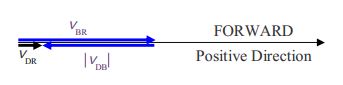
\[\vec{V}_{DR}=\vec{V}_{BR}+\vec{V}_{DB} \nonumber \]
\[V_{DR}=V_{BR}-|V_{DB}| \nonumber \]
\[V_{DR}=55mph-45mph \nonumber \]
\[V_{DR}=10mph \nonumber \]
\(\vec{V}_{DR}=10mph\) in the direction in which the bus is traveling
It would be odd looking at that dart from the side of the road. Relative to you it would still be moving in the direction that the bus is traveling, tail first, at \(10 mph\).
The next easiest kind of vector addition problem is the kind in which the vectors to be added are at right angles to each other. Let’s consider a relative velocity problem involving that kind of vector addition problem.
A boy sitting in a car that is traveling due north at \(65 mph\) aims a BB gun (a gun which uses a compressed gas to fire a small metal or plastic ball called a BB), with a muzzle velocity of \(185 mph\), due east, and pulls the trigger. Recoil (the backward movement of the gun resulting from the firing of the gun) is negligible. In what compass direction does the BB go?
Defining
- \(\vec{V}_{CR}\) to be the velocity of the car relative to the road,
- \(\vec{V}_{BC}\) to be the velocity of the BB relative to the car, and
- \(\vec{V}_{BR}\) to be the velocity of the BB relative to the road; we have
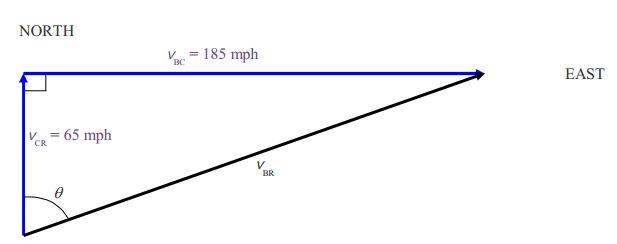
\[tan\theta=\dfrac{V_{BC}}{V_{CR}} \nonumber \]
\[\theta=tan^{-1}\dfrac{V_{BC}}{V_{CR}} \nonumber \]
\[\theta=tan^{-1}\dfrac{185 mph}{65 mph} \nonumber \]
\[\theta=70.6^\circ \nonumber \]
The BB travels in the direction for which the compass heading is \(70.6^\circ\).
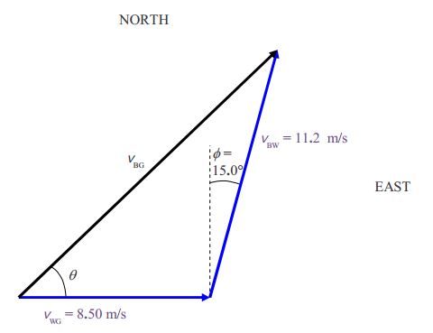
A boat is traveling across a river that flows due east at \(8.50 m/s\). The compass heading of the boat is \(15.0^\circ\). Relative to the water, the boat is traveling straight forward (in the direction in which the boat is pointing) at \(11.2 m/s\). How fast and which way is the boat moving relative to the banks of the river?
Okay, here we have a situation in which the boat is being carried downstream by the movement of the water at the same time that it is moving relative to the water. Note the given information means that if the water was dead still, the boat would be going 11.2 m/s at \(15.0^\circ\) East of North. The water, however, is not still. Defining
- \(\vec{V}_{WG}\) to be the velocity of the water relative to the ground,
- \(\vec{V}_{BW}\) to be the velocity of the boat relative to the water, and
- \(\vec{V}_{BG}\) to be the velocity of the boat relative to the ground; we have
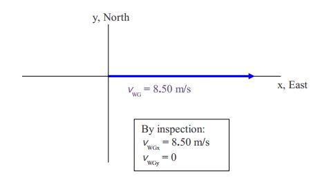
Solving this problem is just a matter of following the vector addition recipe. First we define \(+x\) to be eastward and \(+y\) to be northward. Then we draw the vector addition diagram for \(\vec{V}_{WG}\). Breaking it up into components is trivial since it lies along the x-axis:
Breaking \(\vec{V}_{BW}\) does involve a little bit of work:
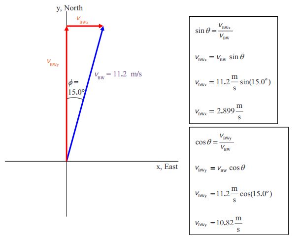
Now we add the \(x\) components to get the \(x\)-component of the resultant
\[V_{BGx}=V_{WGx}+V_{BWx} \nonumber \]
\[V_{BGx}=8.50\dfrac{m}{s}+2.899\dfrac{m}{s} \nonumber \]
\[V_{BGx}=11.299\dfrac{m}{s} \nonumber \]
and we add the y components to get the y-component of the resultant:
\[V_{BGy}=V_{WGy}+V_{BWy} \nonumber \]
\[V_{BGy}=0\dfrac{m}{s}+10.82\dfrac{m}{s} \nonumber \]
\[V_{BGy}=10.82\dfrac{m}{s} \nonumber \]
Now we have both components of the velocity of the boat relative to the ground. We need to draw the vector component diagram for \(\vec{V}_{BG}\) to determine the direction and magnitude of the velocity of the boat relative to the ground.
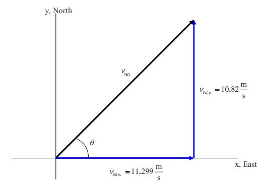
We then use the Pythagorean Theorem to get the magnitude of the velocity of the boat relative to the ground,
\[\vec{V}_{BG}=\sqrt{V_{BGx}^2+V_{BGy}^2} \nonumber \]
\[\vec{V}_{BG}=\sqrt{(11.299m/s)^2+(10.82m/s)^2} \nonumber \]
\[\vec{V}_{BG}=15.64m/s \nonumber \]
and the definition of the tangent to determine the direction of \(\vec{V}_{BG}\):
\[tan\theta=\dfrac{V_{BGy}}{V_{BGx}} \nonumber \]
\[\theta=tan^{-1}\dfrac{V_{BGy}}{V_{BGx}} \nonumber \]
\[\theta=tan^{-1}\dfrac{10.82m/s}{11.299m/s} \nonumber \]
\[\theta=43.8^\circ \nonumber \]
Hence, \(\vec{V}_{BG}=15.64m/s\) at \(43.8^\circ\) North of East.