B32: Calculating the Electric Field from the Electric Potential

The plan here is to develop a relation between the electric field and the corresponding electric potential that allows you to calculate the electric field from the electric potential.

The electric field is the force-per-charge associated with empty points in space that have a forceper- charge because they are in the vicinity of a source charge or some source charges. The electric potential is the potential energy-per-charge associated with the same empty points in space. Since the electric field is the force-per-charge, and the electric potential is the potential energy-per-charge, the relation between the electric field and its potential is essentially a special case of the relation between any force and its associated potential energy. So, I’m going to start by developing the more general relation between a force and its potential energy, and then move on to the special case in which the force is the electric field times the charge of the victim and the potential energy is the electric potential times the charge of the victim.

The idea behind potential energy was that it represented an easy way of getting the work done by a force on a particle that moves from point $A$ to point $B$ under the influence of the force. By definition, the work done is the force along the path times the length of the path. If the force along the path varies along the path, then we take the force along the path at a particular point on the path, times the length of an infinitesimal segment of the path at that point, and repeat, for every infinitesimal segment of the path, adding the results as we go along. The final sum is the work. The potential energy idea represents the assignment of a value of potential energy to every point in space so that, rather than do the path integral just discussed, we simply subtract the value of the potential energy at point $A$ from the value of the potential energy at point $B$. This gives us the change in the potential energy experienced by the particle in moving from point $A$ to point $B$. Then, the work done is the negative of the change in potential energy. For this to be the case, the assignment of values of potential energy values to points in space must be done just right. For things to work out on a macroscopic level, we must ensure that they are correct at an infinitesimal level. We can do this by setting:

$$\mbox{Work as Change in Potential Energy= Work as Force-Along-Path times Path Length} \nonumber$$

$$-dU=\vec{F}\cdot \vec{ds} \nonumber$$

where:

• $dU$ is an infinitesimal change in potential energy,
• $\vec{F}$ is a force, and
• $\vec{ds}$ is the infinitesimal displacement-along-the-path vector.

In Cartesian unit vector notation, $\vec{ds}$ can be expressed as $\vec{ds}=dx \hat{i}+dy \hat{j}+dz\hat{k}$, and $\vec{F}$ can be expressed as $\vec{F}=F_x\hat{i}+F_y\hat{j}+F_z\hat{k}$. Substituting these two expressions into our expression $-dU=\vec{F}\cdot\vec{ds}$, we obtain:

$$-dU=(F_x\hat{i}+F_y\hat{j}+F_z\hat{k})\cdot (dx\hat{i}+dy\hat{j}+dz\hat{k}) \nonumber$$

$$-dU=F_x dx+F_y dy+F_z dz \nonumber$$

Now check this out. If we hold $y$ and $z$ constant (in other words, if we consider $dy$ and $dz$ to be zero) then:

$$\underbrace{-dU=F_x dx}_{ \mbox{when y and z are held constant}} \nonumber$$

Dividing both sides by $dx$ and switching sides yields:

$$\underbrace{F_x=-\frac{dU}{dx}}_{ \mbox{when y and z are held contsant}} \nonumber$$

That is, if you have the potential energy as a function of $x$, $y$, and $z$; and; you take the negative of the derivative with respect to $x$ while holding y and z constant, you get the $x$ component of the force that is characterized by the potential energy function. Taking the derivative of $U$ with respect to $x$ while holding the other variables constant is called taking the partial derivative of $U$ with respect to $x$ and written

$$\frac{\partial U}{\partial x} \nonumber$$

Alternatively, one writes

$$\frac{\partial U}{\partial x}\Big|_{y,z} \nonumber$$

to be read, “the partial derivative of $U$ with respect to $x$ holding $y$ and $z$ constant.” This latter expression makes it more obvious to the reader just what is being held constant. Rewriting our expression for $F_x$ with the partial derivative notation, we have:

$$F_x=-\frac{\partial U}{\partial x} \nonumber$$

Returning to our expression $-dU=F_x dx+F_y dy+F_z dz$, if we hold $x$ and $z$ constant we get:

$$F_y=-\frac{\partial U}{\partial y} \nonumber$$

and, if we hold $x$ and $y$ constant we get,

$$F_z=-\frac{\partial U}{\partial z} \nonumber$$

Substituting these last three results into the force vector expressed in unit vector notation:

$$\vec{F}=F_x \hat{i}+F_y \hat{j}+F_z \hat{k} \nonumber$$

yields

$$\vec{F}=-\frac{\partial U}{\partial x}\hat{i}-\frac{\partial U}{\partial y}\hat{j}-\frac{\partial U}{\partial z}\hat{k} \nonumber$$

which can be written:

$$\vec{F}=-\Big(\frac{\partial U}{\partial x}\hat{i}+\frac{\partial U}{\partial y}\hat{j}+\frac{\partial U}{\partial z}\hat{k}\Big) \nonumber$$

Okay, now, this business of:

• taking the partial derivative of $U$ with respect to $x$ and multiplying the result by the unit vector $\hat{i}$ and then,
• taking the partial derivative of $U$ with respect to $y$ and multiplying the result by the unit vector $\hat{j}$ and then,
• taking the partial derivative of $U$ with respect to $z$ and multiplying the result by the unit vector $\hat{k}$, and then,
• adding all three partial-derivative-times-unit-vector quantities up,

is called “taking the gradient of $U$ “ and is written $\nabla U$. “Taking the gradient” is something that you do to a scalar function, but, the result is a vector. In terms of our gradient notation, we can write our expression for the force as,

$$\vec{F}=-\nabla U \label{32-1}$$

Check this out for the gravitational potential near the surface of the earth. Define a Cartesian coordinate system with, for instance, the origin at sea level, and, with the $x$-$y$ plane being horizontal and the $+z$ direction being upward. Then, the potential energy of a particle of mass $m$ is given as:

$$U=mgz \nonumber$$

Now, suppose you knew this to be the potential but you didn’t know the force. You can calculate the force using $\vec{F}=-\nabla U$, which, as you know, can be written:

$$\vec{F}=-\Big(\frac{\partial U}{\partial x}\hat{i}+\frac{\partial U}{\partial y}\hat{j}+\frac{\partial U}{\partial z} \hat{k}\Big) \nonumber$$

Substituting $U=mgz$ in for $U$ we have

$$\vec{F}=-\Big(\frac{\partial}{\partial x}(mgz)\hat{i}+\frac{\partial}{\partial y}(mgz)\hat{j}+\frac{\partial}{\partial z}(mgz)\hat{k}\Big) \nonumber$$

Now remember, when we take the partial derivative with respect to $x$ we are supposed to hold $y$ and $z$ constant. (There is no $y$.) But, if we hold $z$ constant, then the whole thing $(mgz)$ is constant. And, the derivative of a constant, with respect to $x$, is $0$. In other words, $\frac{\partial}{\partial x}(mgz)=0$. Likewise, $\frac{\partial}{\partial y}(mgz)=0$. In fact, the only non zero partial derivative in our expression for the force is $\frac{\partial}{\partial z}(mgz)=mg$. So:

$$\vec{F}=-(0\hat{i}+0\hat{j}+mg \hat{k}) \nonumber$$

In other words:

$$\vec{F}=-mg\hat{k} \nonumber$$

That is to say that, based on the gravitational potential $U=mgz$, the gravitational force is in the $\hat{k}$direction (downward), and, is of magnitude mg. Of course, you knew this in advance, the gravitational force in question is just the weight force. The example was just meant to familiarize you with the gradient operator and the relation between force and potential energy.

Okay, as important as it is that you realize that we are talking about a general relationship between force and potential energy, it is now time to narrow the discussion to the case of the electric force and the electric potential energy, and, from there, to derive a relation between the electric field and electric potential (which is electric potential-energy-per-charge).

Starting with $\vec{F}=-\nabla U$ written out the long way:

$$\vec{F}=-\Big(\frac{\partial U}{\partial x}\hat{i}+\frac{\partial U}{\partial y}\hat{j}+\frac{\partial U}{\partial z}\hat{k}\Big) \nonumber$$

we apply it to the case of a particle with charge $q$ in an electric field $\vec{E}$ (caused to exist in the region of space in question by some unspecified source charge or distribution of source charge). The electric field exerts a force $\vec{F}=q\vec{E}$ on the particle, and, the particle has electric potential energy $U=q \varphi$ where $\varphi$ is the electric potential at the point in space at which the charged particle is located. Plugging these into $\vec{F}=-\Big(\frac{\partial U}{\partial x}\hat{i}+\frac{\partial U}{\partial y}\hat{j}+\frac{\partial U}{\partial z}\hat{k}\Big)$ yields:

$$q\vec{E}=-\Big(\frac{\partial (q\varphi)}{\partial x}\hat{i}+\frac{\partial (q\varphi)}{\partial y}\hat{j}+\frac{\partial (q\varphi)}{\partial z}\hat{k}\Big) \nonumber$$

which I copy here for your convenience:

$$q\vec{E}=-\Big( \frac{\partial(q\varphi)}{\partial x}\hat{i}+\frac{\partial (q\varphi)}{\partial y}\hat{j}+\frac{\partial(q\varphi)}{\partial z}\hat{k}\Big) \nonumber$$

The $q$ inside each of the partial derivatives is a constant so we can factor it out of each partial derivative.

$$q\vec{E}=-\Big(q\frac{\partial \varphi}{\partial x}\hat{i}+q\frac{\partial \varphi}{\partial y} \hat{j}+q\frac{\partial \varphi}{\partial z}\hat{k}\Big) \nonumber$$

Then, since $q$ appears in every term, we can factor it out of the sum:

$$q\vec{E}=-q\Big(\frac{\partial \varphi}{\partial x}\hat{i}+\frac{\partial \varphi}{\partial y}\hat{j}+\frac{\partial \varphi}{\partial z}\hat{k}\Big) \nonumber$$

Dividing both sides by the charge of the victim yields the desired relation between the electric field and the electric potential:

$$\vec{E}=-\Big(\frac{\partial \varphi}{\partial x}\hat{i}+\frac{\partial \varphi}{\partial y}\hat{j}+\frac{\partial \varphi}{\partial z}\hat{k}\Big) \nonumber$$

We see that the electric field $\vec{E}$ is just the gradient of the electric potential $\varphi$. This result can be expressed more concisely by means of the gradient operator as:

$$\vec{E}=-\nabla \varphi \label{32-2}$$

In Example 31-1, we found that the electric potential due to a pair of particles, one of charge $+q$ at $(0, d/2)$ and the other of charge $–q$ at $(0, – d/2)$, is given by:

$$\varphi=\frac{kq}{\sqrt{x^2+(y-\frac{d}{2})^2}}-\frac{kq}{\sqrt{x^2+(y+\frac{d}{2})^2}} \nonumber$$

Such a pair of charges is called an electric dipole. Find the electric field of the dipole, valid for any point on the x axis.

Solution: We can use a symmetry argument and our conceptual understanding of the electric field due to a point charge to deduce that the $x$ component of the electric field has to be zero, and, the $y$ component has to be negative. But, let’s use the gradient method to do that, and, to get an expression for the $y$ component of the electric field. I do argue, however that, from our conceptual understanding of the electric field due to a point charge, neither particle’s electric field has a $z$ component in the $x$-$y$ plane, so we are justified in neglecting the $z$ component altogether. As such our gradient operator expression for the electric field

$$\vec{E}=-\nabla \varphi \nonumber$$

becomes

$$\vec{E}=-\Big(\frac{\partial \varphi}{\partial x}\hat{i}+\frac{\partial \varphi}{\partial y}\hat{j}\Big) \nonumber$$

Let’s work on the $\frac{\partial \varphi}{\partial x}$ part:

$$\frac{\partial \varphi}{\partial x}=\frac{\partial}{\partial x} \Big(\frac{kq}{\sqrt{x^2+(y-\frac{d}{2})^2}}-\frac{kq}{\sqrt{x^2+(y+\frac{d}{2})^2}}\Big) \nonumber$$

$$\frac{\partial \varphi}{\partial x}=kq \frac{\partial}{\partial x}\Big(\Big[ x^2+(y-\frac{d}{2})^2\Big]^{-\frac{1}{2}}-\Big[x^2+(y+\frac{d}{2})^2\Big]^{-\frac{1}{2}}\Big) \nonumber$$

$$\frac{\partial \varphi}{\partial x}=kq\Big(-\frac{1}{2}\Big[x^2+(y-\frac{d}{2})^2\Big]^{-\frac{3}{2}}2x-\space -\frac{1}{2} \Big[x^2+(y+\frac{d}{2})^2\Big]^{-\frac{3}{2}}2x\Big) \nonumber$$

$$\frac{\partial \varphi}{\partial x}=kqx \Big(\Big[x^2+(y+\frac{d}{2})^2\Big]^{-\frac{3}{2}}-\Big[x^2+(y-\frac{d}{2})^2\Big]^{-\frac{3}{2}}\Big) \nonumber$$

$$\frac{\partial \varphi}{\partial x}=\frac{kqx}{\Big[x^2+(y+\frac{d}{2})^2\Big]^{\frac{3}{2}}}-\frac{kqx}{\Big[x^2+(y-\frac{d}{2})^2\Big]^{\frac{3}{2}}} \nonumber$$

We were asked to find the electric field on the x axis, so, we evaluate this expression at $y=0$:

$$\frac{\partial \varphi}{\partial x}=\frac{kqx}{\Big[x^2+(0+\frac{d}{2})^2\Big]^{\frac{3}{2}}}-\frac{kqx}{\Big[x^2+(0-\frac{d}{2})^2\Big]^{\frac{3}{2}}} \nonumber$$

$$\frac{\partial \varphi}{\partial x} \Big|_{y=0}=0 \nonumber$$

To continue with our determination of $\vec{E}=-(\frac{\partial \varphi}{\partial x}\hat{i}+\frac{\partial \varphi}{\partial y}\hat{j})$, we next solve for $\frac{\partial \varphi}{\partial y}$.

$$\frac{\partial \varphi}{\partial y}=\frac{\partial}{\partial y} \Big(\frac{kq}{\sqrt{x^2+(y-\frac{d}{2})^2}}-\frac{kq}{\sqrt{x^2+(y+\frac{d}{2})^2}}\Big) \nonumber$$

$$\frac{\partial \varphi}{\partial y}=kq \frac{\partial}{\partial y}\Big(\Big[x^2+(y-\frac{d}{2})^2\Big]^{-\frac{1}{2}}-\Big[x^2+(y+\frac{d}{2})^2 \Big] ^{-\frac{1}{2}}\Big) \nonumber$$

$$\frac{\partial \varphi}{\partial y}=kq \Big(-\frac{1}{2}\Big[x^2+(y-\frac{d}{2})^2\Big]^{-\frac{3}{2}}2(y-\frac{d}{2})-\space-\frac{1}{2}\Big[x^2+(y+\frac{d}{2})^2\Big]^{-\frac{3}{2}}2(y+\frac{d}{2}) \nonumber$$

$$\frac{\partial \varphi}{\partial y}=kq\Big(\Big[x^2+(y+\frac{d}{2})^2\Big]^{-\frac{3}{2}}(y+\frac{d}{2})-\Big[x^2+(y-\frac{d}{2})^2\Big]^{-\frac{3}{2}}(y-\frac{d}{2})\Big) \nonumber$$

$$\frac{\partial \varphi}{\partial y}=\frac{kq(y+\frac{d}{2})}{\Big[ x^2+(y+\frac{d}{2})^2\Big]^{\frac{3}{2}}}-\frac{kq(y-\frac{d}{2})}{\Big[x^2+(y-\frac{d}{2})^2\Big]^{\frac{3}{2}}} \nonumber$$

Again, we were asked to find the electric field on the x axis, so, we evaluate this expression at $y=0$:

$$\frac{\partial \varphi}{\partial y}\Big|_{y=0}=\frac{kq\Big(0+\frac{d}{2}\Big)}{\Big[x^2+\Big(0+\frac{d}{2}\Big)^2\Big]^{\frac{3}{2}}}-\frac{kq\Big(0-\frac{d}{2}\Big)}{\Big[x^2+\Big(0-\frac{d}{2}\Big)^2\Big]^{\frac{3}{2}}} \nonumber$$

$$\frac{\partial\varphi}{\partial y}\Big|_{y=0}=\frac{kqd}{\Big[x^2+\frac{d^2}{4}\Big]^{\frac{3}{2}}} \nonumber$$

Plugging $\frac{\partial \varphi}{\partial x}\Big|_{y=0}=0$ and $\frac{\partial \varphi}{\partial y}\Big|_{y=0}=\frac{kqd}{\Big[x^2+\frac{d^2}{4}\Big]^{\frac{3}{2}}}$ into $\vec{E}=-\Big(\frac{\partial\varphi}{\partial x}\hat{i}+\frac{\partial\varphi}{\partial y}\hat{j}\Big)$ yields:

$$\vec{E}=-\Big(0\hat{i}+\frac{kqd}{[x^2+\frac{d^2}{4}]^{\frac{3}{2}}}\hat{j}\Big) \nonumber$$

$$\vec{E}=-\frac{kqd}{[x^2+\frac{d^2}{4}]^{\frac{3}{2}}}\hat{j} \nonumber$$

As expected, $\vec{E}$ is in the –y direction. Note that to find the electric field on the $x$ axis, you have to take the derivatives first, and then evaluate at $y=0$.

A line of charge extends along the $x$ axis from $x=a$ to $x=b$. On that line segment, the linear charge density $\lambda$ is a constant. Find the electric potential as a function of position ($x$ and $y$) due to that charge distribution on the $x$-$y$ plane, and then, from the electric potential, determine the electric field on the $x$ axis.

Solution: First, we need to use the methods of chapter 31 to get the potential for the specified charge distribution (a linear charge distribution with a constant linear charge density $\lambda$ ).

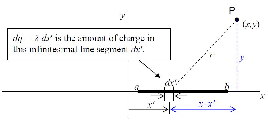
$$d \varphi=\frac{k\space dq}{r} \nonumber$$

$$dq=\lambda dx' \quad \mbox{and} \quad r=\sqrt{(r-x')^2+y^2} \nonumber$$

$$d\varphi=\frac{k\lambda (x')dx'}{\sqrt{(x-x')^2+y^2}} \nonumber$$

$$\int d\varphi=\int_{a}^{b} \frac{k\lambda dx'}{\sqrt{(x-x')^2+y^2}} \nonumber$$

$$\varphi=k\lambda \int_{a}^{b} \frac{dx'}{\sqrt{(x-x')^2+y^2}} \nonumber$$

To carry out the integration, we use the variable substitution:

$$u=x-x' \nonumber$$

$$du=-dx' \Rightarrow dx'=du \nonumber$$

Lower Integration Limit: When

$$x'=a, u=x-a \nonumber$$

Upper Integration Limit: When

$$x'=b, u=x-b \nonumber$$

Making these substitutions, we obtain:

$$\varphi=k\lambda \int_{x-a}^{x-b} \frac{-du}{\sqrt{u^2+y^2}} \nonumber$$

which I copy here for your convenience:

$$\varphi=k\lambda \int_{x-a}^{x-b} \frac{-du}{\sqrt{u^2+y^2}} \nonumber$$

Using the minus sign to interchange the limits of integration, we have:

$$\varphi=k\lambda \int_{x-a}^{x-b} \frac{du}{\sqrt{u^2+y^2}} \nonumber$$

Using the appropriate integration formula from the formula sheet we obtain:

$$\varphi=k\lambda \ln(u+\sqrt{u^2+y^2}) \Big|_{x-b}^{x-a} \nonumber$$

$$\varphi=k\lambda \Big\{ \ln[ x-a+\sqrt{(x-a)^2+y^2} \space\Big] -\ln \Big[x-b+\sqrt{(x-b)^2+y^2}\space\Big] \Big\} \nonumber$$

Okay, that’s the potential. Now we have to take the gradient of it and evaluate the result at $y = 0$ to get the electric field on the x axis. We need to find

$$\vec{E}=-\bigtriangledown \varphi \nonumber$$

which, in the absence of any $z$ dependence, can be written as:

$$\vec{E}=-\Big( \frac{\partial \varphi}{\partial x}\hat{i}+\frac{\partial \varphi}{\partial y}\hat{j} \Big) \nonumber$$

We start by finding $\frac{\partial \varphi}{\partial x}$:

$$\frac{\partial \varphi}{\partial x}=\frac{\partial}{\partial x}\Big( k\lambda \Big\{\ln \Big[x-a+\sqrt{(x-a)^2+y^2} \, \Big]-\ln \Big[x-b+\sqrt{(x-b)^2+y^2} \space\Big] \Big\} \Big) \nonumber$$

$$\frac{\partial \varphi}{\partial x}=k\lambda \Big\{ \frac{\partial}{\partial x}\ln \Big[ x-a+((x-a)^2+y^2)^{\frac{1}{2}}\Big] -\frac{\partial}{\partial x}\ln \Big[x-b+((x-b)^2+y^2)^{\frac{1}{2}}\Big] \Big\} \nonumber$$

$$\frac{\partial \varphi}{\partial x}=k\lambda \Bigg\{ \frac{1+\frac{1}{2}\Big( (x-a)^2+y^2\Big) ^{-\frac{1}{2}} 2(x-a)}{x-a+\Big( (x-a)^2+y^2\Big)^{\frac{1}{2}}}-\frac{1+\frac{1}{2}\Big( (x-b)^2+y^2\Big) ^{-\frac{1}{2}} 2(x-b)}{x-b+\Big( (x-b)^2+y^2\Big)^{\frac{1}{2}}}\Bigg\} \nonumber$$

$$\frac{\partial \varphi}{\partial x}=k\lambda \Bigg\{\frac{1+(x-a)\Big((x-a)^2+y^2\Big)^{-\frac{1}{2}}}{x-a+\Big( (x-a)^2+y^2 \Big)^{\frac{1}{2}}}-\frac{1+(x-b)\Big((x-b)^2+y^2\Big)^{-\frac{1}{2}}}{x-b+\Big( (x-b)^2+y^2 \Big)^{\frac{1}{2}}} \Bigg\} \nonumber$$

Evaluating this at $y=0$ yields:

$$\frac{\partial \varphi}{\partial x} \Big|_{y=0}=k\lambda \Big(\frac{1}{x-a}-\frac{1}{x-b} \Big) \nonumber$$

Now, let’s work on getting $\frac{\partial \varphi}{\partial y}$. I’ll copy our result for $\varphi$ from above and then take the partial derivative with respect to $y$ (holding $x$ constant):

$$\varphi=k\lambda \Bigg\{ \ln \Big[ x-a+\sqrt{(x-a)^2+y^2} \, \Big]-\ln \Big[ x-b+\sqrt{(x-b)^2+y^2} \, \Big] \Bigg\} \nonumber$$

$$\frac{\partial \varphi}{\partial y}=\frac{\partial}{\partial y} \Bigg( k\lambda \Big\{ \ln\Big[x-a+\sqrt{(x-a)^2+y^2}\space \Big]- \ln\Big[x-b+\sqrt{(x-b)^2+y^2}\space \Big] \Big\} \Bigg) \nonumber$$

$$\frac{\partial \varphi}{\partial y}=k\lambda \Bigg\{ \frac{\partial}{\partial y} \ln \Big[x-a+\Big((x-a)^2+y^2 \Big)^{\frac{1}{2}} \Big]- \frac{\partial}{\partial x} \ln \Big[x-b+\Big((x-b)^2+y^2 \Big)^{\frac{1}{2}} \Big] \Bigg\} \nonumber$$

$$\frac{\partial \varphi}{\partial y}=k\lambda \Bigg\{ \frac{\frac{1}{2}\Big((x-a)^2+y^2 \Big)^{-\frac{1}{2}} 2y}{x-a+\Big( (x-a)^2+y^2\Big)^{\frac{1}{2}}}-\frac{\frac{1}{2}\Big((x-b)^2+y^2 \Big)^{-\frac{1}{2}} 2y}{x-b+\Big( (x-b)^2+y^2\Big)^{\frac{1}{2}}} \Bigg\} \nonumber$$

$$\frac{\partial \varphi}{\partial y}=k\lambda \Bigg\{ \frac{y\Big((x-a)^2+y^2 \Big)^{-\frac{1}{2}}}{x-a+\Big( (x-a)^2+y^2\Big)^{\frac{1}{2}}}-\frac{y\Big((x-b)^2+y^2 \Big)^{-\frac{1}{2}}}{x-b+\Big( (x-b)^2+y^2\Big)^{\frac{1}{2}}} \Bigg\} \nonumber$$

Evaluating this at $y=0$ yields:

$$\frac{\partial \varphi}{\partial y} \Big|_{y=0} =0 \nonumber$$

Plugging $\frac{\partial \varphi}{\partial x} \Big|_{y=0} =k\lambda \Big( \frac{1}{x-a}-\frac{1}{x-b}\Big)$ and $\frac{\partial \varphi}{\partial y} \Big|_{y=0} =0$ into $\vec{E}=-\Big(\frac{\partial \varphi}{\partial x}\hat{i}+\frac{\partial \varphi}{\partial y}\hat{j}\Big)$ yields:

$$\vec{E}=-\Big( k \lambda \Big(\frac{1}{x-a}-\frac{1}{x-b} \Big)\hat{i}+0 \hat{j} \Big) \nonumber$$

$$\vec{E}=k \lambda\Big(\frac{1}{x-b}-\frac{1}{x-a}\Big) \hat{i} \nonumber$$