Physics LibreTexts

9.8: Problem Solving

  • Page ID
    15514
  • \( \newcommand{\vecs}[1]{\overset { \scriptstyle \rightharpoonup} {\mathbf{#1}} } \)

    \( \newcommand{\vecd}[1]{\overset{-\!-\!\rightharpoonup}{\vphantom{a}\smash {#1}}} \)

    \( \newcommand{\id}{\mathrm{id}}\) \( \newcommand{\Span}{\mathrm{span}}\)

    ( \newcommand{\kernel}{\mathrm{null}\,}\) \( \newcommand{\range}{\mathrm{range}\,}\)

    \( \newcommand{\RealPart}{\mathrm{Re}}\) \( \newcommand{\ImaginaryPart}{\mathrm{Im}}\)

    \( \newcommand{\Argument}{\mathrm{Arg}}\) \( \newcommand{\norm}[1]{\| #1 \|}\)

    \( \newcommand{\inner}[2]{\langle #1, #2 \rangle}\)

    \( \newcommand{\Span}{\mathrm{span}}\)

    \( \newcommand{\id}{\mathrm{id}}\)

    \( \newcommand{\Span}{\mathrm{span}}\)

    \( \newcommand{\kernel}{\mathrm{null}\,}\)

    \( \newcommand{\range}{\mathrm{range}\,}\)

    \( \newcommand{\RealPart}{\mathrm{Re}}\)

    \( \newcommand{\ImaginaryPart}{\mathrm{Im}}\)

    \( \newcommand{\Argument}{\mathrm{Arg}}\)

    \( \newcommand{\norm}[1]{\| #1 \|}\)

    \( \newcommand{\inner}[2]{\langle #1, #2 \rangle}\)

    \( \newcommand{\Span}{\mathrm{span}}\) \( \newcommand{\AA}{\unicode[.8,0]{x212B}}\)

    \( \newcommand{\vectorA}[1]{\vec{#1}}      % arrow\)

    \( \newcommand{\vectorAt}[1]{\vec{\text{#1}}}      % arrow\)

    \( \newcommand{\vectorB}[1]{\overset { \scriptstyle \rightharpoonup} {\mathbf{#1}} } \)

    \( \newcommand{\vectorC}[1]{\textbf{#1}} \)

    \( \newcommand{\vectorD}[1]{\overrightarrow{#1}} \)

    \( \newcommand{\vectorDt}[1]{\overrightarrow{\text{#1}}} \)

    \( \newcommand{\vectE}[1]{\overset{-\!-\!\rightharpoonup}{\vphantom{a}\smash{\mathbf {#1}}}} \)

    \( \newcommand{\vecs}[1]{\overset { \scriptstyle \rightharpoonup} {\mathbf{#1}} } \)

    \( \newcommand{\vecd}[1]{\overset{-\!-\!\rightharpoonup}{\vphantom{a}\smash {#1}}} \)

    \(\newcommand{\avec}{\mathbf a}\) \(\newcommand{\bvec}{\mathbf b}\) \(\newcommand{\cvec}{\mathbf c}\) \(\newcommand{\dvec}{\mathbf d}\) \(\newcommand{\dtil}{\widetilde{\mathbf d}}\) \(\newcommand{\evec}{\mathbf e}\) \(\newcommand{\fvec}{\mathbf f}\) \(\newcommand{\nvec}{\mathbf n}\) \(\newcommand{\pvec}{\mathbf p}\) \(\newcommand{\qvec}{\mathbf q}\) \(\newcommand{\svec}{\mathbf s}\) \(\newcommand{\tvec}{\mathbf t}\) \(\newcommand{\uvec}{\mathbf u}\) \(\newcommand{\vvec}{\mathbf v}\) \(\newcommand{\wvec}{\mathbf w}\) \(\newcommand{\xvec}{\mathbf x}\) \(\newcommand{\yvec}{\mathbf y}\) \(\newcommand{\zvec}{\mathbf z}\) \(\newcommand{\rvec}{\mathbf r}\) \(\newcommand{\mvec}{\mathbf m}\) \(\newcommand{\zerovec}{\mathbf 0}\) \(\newcommand{\onevec}{\mathbf 1}\) \(\newcommand{\real}{\mathbb R}\) \(\newcommand{\twovec}[2]{\left[\begin{array}{r}#1 \\ #2 \end{array}\right]}\) \(\newcommand{\ctwovec}[2]{\left[\begin{array}{c}#1 \\ #2 \end{array}\right]}\) \(\newcommand{\threevec}[3]{\left[\begin{array}{r}#1 \\ #2 \\ #3 \end{array}\right]}\) \(\newcommand{\cthreevec}[3]{\left[\begin{array}{c}#1 \\ #2 \\ #3 \end{array}\right]}\) \(\newcommand{\fourvec}[4]{\left[\begin{array}{r}#1 \\ #2 \\ #3 \\ #4 \end{array}\right]}\) \(\newcommand{\cfourvec}[4]{\left[\begin{array}{c}#1 \\ #2 \\ #3 \\ #4 \end{array}\right]}\) \(\newcommand{\fivevec}[5]{\left[\begin{array}{r}#1 \\ #2 \\ #3 \\ #4 \\ #5 \\ \end{array}\right]}\) \(\newcommand{\cfivevec}[5]{\left[\begin{array}{c}#1 \\ #2 \\ #3 \\ #4 \\ #5 \\ \end{array}\right]}\) \(\newcommand{\mattwo}[4]{\left[\begin{array}{rr}#1 \amp #2 \\ #3 \amp #4 \\ \end{array}\right]}\) \(\newcommand{\laspan}[1]{\text{Span}\{#1\}}\) \(\newcommand{\bcal}{\cal B}\) \(\newcommand{\ccal}{\cal C}\) \(\newcommand{\scal}{\cal S}\) \(\newcommand{\wcal}{\cal W}\) \(\newcommand{\ecal}{\cal E}\) \(\newcommand{\coords}[2]{\left\{#1\right\}_{#2}}\) \(\newcommand{\gray}[1]{\color{gray}{#1}}\) \(\newcommand{\lgray}[1]{\color{lightgray}{#1}}\) \(\newcommand{\rank}{\operatorname{rank}}\) \(\newcommand{\row}{\text{Row}}\) \(\newcommand{\col}{\text{Col}}\) \(\renewcommand{\row}{\text{Row}}\) \(\newcommand{\nul}{\text{Nul}}\) \(\newcommand{\var}{\text{Var}}\) \(\newcommand{\corr}{\text{corr}}\) \(\newcommand{\len}[1]{\left|#1\right|}\) \(\newcommand{\bbar}{\overline{\bvec}}\) \(\newcommand{\bhat}{\widehat{\bvec}}\) \(\newcommand{\bperp}{\bvec^\perp}\) \(\newcommand{\xhat}{\widehat{\xvec}}\) \(\newcommand{\vhat}{\widehat{\vvec}}\) \(\newcommand{\uhat}{\widehat{\uvec}}\) \(\newcommand{\what}{\widehat{\wvec}}\) \(\newcommand{\Sighat}{\widehat{\Sigma}}\) \(\newcommand{\lt}{<}\) \(\newcommand{\gt}{>}\) \(\newcommand{\amp}{&}\) \(\definecolor{fillinmathshade}{gray}{0.9}\)

    learning objectives

    • Develop and apply a strong problem-solving strategy for rotational kinematics

    Problem-Solving Strategy For Rotational Kinematics

    When solving problems on rotational kinematics:

    • Examine the situation to determine that rotational kinematics (rotational motion) is involved. Rotation must be involved, but without the need to consider forces or masses that affect the motion.
    • Identify exactly what needs to be determined in the problem (identify the unknowns). A sketch of the situation is useful.
    • Make a list of what is given or can be inferred from the problem as stated (identify the knowns).
    • Solve the appropriate equation or equations for the quantity to be determined (the unknown). It can be useful to think in terms of a translational analog because by now you are familiar with such motion.
    • Substitute the known values along with their units into the appropriate equation, and obtain numerical solutions complete with units. Be sure to use units of radians for angles.
    • Check your answer to see if it is reasonable: Does your answer make sense?

    Example \(\PageIndex{1}\):

    Suppose a large freight train accelerates from rest, giving its 0.350 m radius wheels an angular acceleration of 0.250 rad/s2. After the wheels have made 200 revolutions (assume no slippage): (a) How far has the train moved down the track? (b) What are the final angular velocity of the wheels and the linear velocity of the train?

    In part (a), we are asked to find x, and in (b) we are asked to find ω and v. We are given the number of revolutions θ, the radius of the wheels r, and the angular acceleration α.

    The distance x is very easily found from the relationship between distance and rotation angle: \(\mathrm{θ=\frac{x}{r}}\).

    Solving this equation for x yields \(\mathrm{x=rθ}\).

    Before using this equation, we must convert the number of revolutions into radians, because we are dealing with a relationship between linear and rotational quantities:

    \[\mathrm{θ=(200 rev)(\dfrac{2π \; rad}{1 \; rev})=1257 \; rad.}\]

    Substitute the known values into \(\mathrm{x=rθ}\) to find the distance the train moved down the track:

    \[\mathrm{x=rθ=(0.350 \;m)(1257 \; rad)=440 \; m.}\]

    We cannot use any equation that incorporates t to find ω, because the equation would have at least two unknown values. The equation \(\mathrm{ω^2=ω_0^2+2 \alpha \theta}\) will work, because we know the values for all variables except ω. Taking the square root of this equation and entering the known values gives

    \[\begin{align} \mathrm{ω} & \mathrm{=\sqrt{0+2(0.250 \; rad/s^2)(1257 \; rad)}} \\ & \mathrm{=25.1 \; rad/s} \end{align}\]

    One may find the linear velocity of the train, v, through its relationship to ω:

    \[\mathrm{v=rω=(0.350 \; m)(25.1 \; rad/s)=8.77 \; m/s}\]

    Rotational motion: Part of a series of videos on physics problem-solving. The problems are taken from “The Joy of Physics. ” This one deals with angular motion. The viewer is urged to pause the video at the problem statement and work the problem before watching the rest of the video.
    image

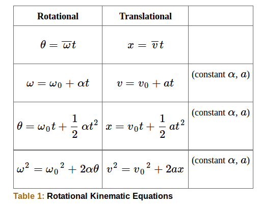
    Equation list: Rotational and translational kinematic equations.

    Key Points

    • Examine the situation to determine that rotational kinematics (rotational motion ) is involved, and identify exactly what needs to be determined.
    • Make a list of what is given or can be inferred from the problem as stated and solve the appropriate equations.
    • Substitute the known values along with their units into the appropriate equation, and obtain numerical solutions complete with units.

    Key Terms

    • kinematics: The branch of mechanics concerned with objects in motion, but not with the forces involved.

    LICENSES AND ATTRIBUTIONS

    CC LICENSED CONTENT, SHARED PREVIOUSLY

    CC LICENSED CONTENT, SPECIFIC ATTRIBUTION


    9.8: Problem Solving is shared under a not declared license and was authored, remixed, and/or curated by LibreTexts.