1.5: Exponential Solutions

We are now ready to translate the conditions of linearity and time translation invariance into mathematics. What we will see is that the two properties of linearity and time translation invariance lead automatically to irreducible solutions satisfying (1.38), and furthermore that

Figure 1.8: Some special complex exponential in the complex plane.

these irreducible solutions are just exponential. We do not need to use any other details about the equation of motion to get this result. Therefore our arguments will apply to much more complicated situations, in which there is damping or more degrees of freedom or both. So long as the system has time translation invariance and linearity, the solutions will be sums of irreducible exponential solutions.

We have seen that the solutions of homogeneous linear differential equations with constant coefficients, of the form,

\[M\frac{d^2}{dt^2} x(t) + K x(t) = 0,\]

have the properties of linearity and time translation invariance. The equation of simple harmonic motion is of this form. The coordinates are real, and the constants \(M\) and \(K\) are real because they are physical things like masses and spring constants. However, we want to allow ourselves the luxury of considering complex solutions as well, so we consider the same equation with complex variables:

\[M\frac{d^2}{dt^2} z(t) + K z(t) = 0.\]

Note the relation between the solutions to (1.68) and (1.69). Because the coefficients \(M\) and \(K\) are real, for every solution, \(z(t)\), of (1.69), the complex conjugate, \(z(t)^*\), is also a solution. The differential equation remains true when the signs of all the \(i\)’s are changed.

From these two solutions, we can construct two real solutions:

\[x_1(t) = Re (z(t)) = (z(t) + z(t)^*) /2 ;\]

\[x_2(t) = Im (z(t)) = (z(t) − z(t)^*) /2i.\]

All this is possible because of linearity, which allows us to go back and forth from real to complex solutions by forming linear combinations, as in (1.70). These are solutions of (1.68). Note that \(x_1(t)\) and \(x_2(t)\) are just the real and imaginary parts of \(z(t)\). The point is that you can always reconstruct the physical real solutions to the equation of motion from the complex solution. You can do all of the mathematics using complex variables, which makes it much easier. Then at the end you can get the physical solution of interest just by taking the real part of your complex solution.

Now back to the solution to (1.69). What we want to show is that we are led to irreducible, exponential solutions for any system with time translation invariance and linearity! Thus we will understand why we can always find irreducible solutions, not only in (1.69), but in much more complicated situations with damping, or more degrees of freedom.

There are two crucial elements:

1. Time translation invariance, (1.33), which requires that \(x(t + a)\) is a solution if \(x(t)\) is a solution;
2. Linearity, which allows us to form linear combinations of solutions to get new solutions.

We will solve (1.68) using only these two elements. That will allow us to generalize our solution immediately to any system in which the properties, (1.71), are present.

One way of using linearity is to choose a “basis” set of solutions, \(x_j (t)\) for \(j = 1\) to \(n\) which is “complete” and “linearly independent.” For the harmonic oscillator, two solutions are all we need, so \(n = 2.\) But our analysis will be much more general and will apply, for example, to linear systems with more degrees of freedom, so we will leave \(n\) free. What “complete” means is that any solution, \(z(t)\), (which may be complex) can be expressed as a linear combination of the \(x_j (t)\)’s,

\[z(t) = \displaystyle \sum_{j=1}^n c_jx_j(t).\]

What “linearly independent” means is that none of the \(x_j (t)\)’s can be expressed as a linear combination of the others, so that the only linear combination of the \(x_j (t)\)’s that vanishes is the trivial combination, with only zero coefficients,

\[\displaystyle \sum_{j=1}^n c_jx_j(t) = 0 ⇒ c_j = 0.\]

Now let us see whether we can find an irreducible solution that behaves simply under a change in the initial clock setting, as in (1.38),

\[z(t + a) = h(a) z(t)\]

for some (possibly complex) function \(h(a)\). In terms of the basis solutions, this is

\[z(t + a) = h(a) \displaystyle \sum_{k=1}^n c_kx_k(t).\]

But each of the basis solutions also goes into a solution under a time translation, and each new solution can, in turn, be written as a linear combination of the basis solutions, as follows:

\[x_j(t + a) = \displaystyle \sum_{k=1}^n R_{jk}(a)x_k(t).\]

Thus

\[z(t + a) = \displaystyle \sum_{j=1}^n c_jx_j(t+a) = \displaystyle \sum_{j,k=1}^n c_jR_{jk}(a)x_k(t).\]

Comparing (1.75) and (1.77), and using (1.73), we see that we can find an irreducible solution if and only if

\[\displaystyle \sum_{j=1}^n c_jR_{jk}(a) = h(a) c_k for all k.\]

This is called an “eigenvalue equation.” We will have much more to say about eigenvalue equations in chapter 3, when we discuss matrix notation. For now, note that (1.78) is a set of \(n\) homogeneous simultaneous equations in the \(n\) unknown coefficients, \(c_j\). We can rewrite it as

\[\displaystyle \sum_{j=1}^n c_jS_{jk}(a) = 0 for all k,\]

where

\[S_{jk}(a) = \begin{cases} R_{jk}(a) for j =/ k, \\ R_{jk}(a) - h(a) for j = k. \end{cases}\]

We can find a solution to (1.78) if and only if there is a solution of the determinantal equation⁵

\[det S_{jk}(a) = 0.\]

___________________________

⁵We will discuss the determinant in detail in chapter 3, so if you have forgotten this result from algebra, don’t worry about it for now.

(1.81) is an \(n\)th order equation in the variable \(h(a)\). It may have no real solution, but it always has \(n\) complex solutions for \(h(a)\) (although some of the \(h(a)\) values may appear more than once). For each solution for \(h(a)\), we can find a set of \(c_j\)s satisfying (1.78). The different linear combinations, \(z(t)\), constructed in this way will be a linearly independent set of irreducible solutions, each satisfying (1.74), for some \(h(a)\). If there are \(n\) different \(h(a)\)s, the usual situation, they will be a complete set of irreducible solutions to the equations of motions. Then we may as well take our solutions to be irreducible, satisfying (1.74). We will see later what happens when some of the \(h(a)\)s appear more than once so that there are fewer than \(n\) different ones.

Now for each such irreducible solution, we can see what the functions \(h(a)\) and \(z(a)\) must be. If we differentiate both sides of (1.74) with respect to \(a\), we obtain

\[z' (t + a) = h' (a) z(t).\]

Setting \(a = 0\) gives

\[z' (t) = H z(t)\]

where

\[H ≡ h' (0).\]

This implies

\[z(t) ∝ e^{Ht} .\]

Thus the irreducible solution is an exponential! We have shown that (1.71) leads to irreducible, exponential solutions, without using any of details of the dynamics!

Building Up The Exponential

There is another way to see what (1.74) implies for the form of the irreducible solution that does not even involve solving the simple differential equation, (1.83). Begin by setting \(t=0\) in (1.74). This gives

\[h(a) = z(a)/z(0).\]

\(h(a)\) is proportional to \(z(a)\). This is particularly simple if we choose to multiply our irreducible solution by a constant so that \(z(0) = 1\). Then (1.86) gives

\[h(a) = z(a)\]

and therefore

\[z(t + a) = z(t) z(a).\]

Consider what happens for very small \(t = ϵ << 1\). Performing a Taylor expansion, we can write

\[z(ϵ) = 1 + Hϵ + O(ϵ^2)\]

where H = z'(0) from (1.84) and (1.87). Using (1.88), we can show that

\[z(Nϵ) = [z(ϵ)]^N.\]

Then for any \(t\) we can write (taking t = N?)

\[z(t) = \displaystyle \lim_{N \to \infty}[z(t/N)]^N = \displaystyle \lim_{N\to \infty}[1+H(t/N)]^N = e^{(Ht)}\]

Thus again, we see that the irreducible solution with respect to time translation invariance is just an exponential! 6

\[z(t) = e^{Ht}\].

What is H?

When we put the irreducible solution, \(e^{Ht}\), into (1.69), the derivatives just pull down powers of H so the equation becomes a purely algebraic equation (dropping an overall factor of \(e^{Ht}\))

\[MH^2 + K = 0\]

Now, finally, we can see the relevance of complex numbers to the above discussion of time translation invariance. For positive M and K, the equation (1.93) has no solutions at all if we restrict H to be real. We cannot find any real irreducible solutions. But there are always two solutions for H in the complex numbers. In this case, the solution is

\[H=±iw\] where \[w=sqrt{\frac{K}{M}}\]

It is only in this last step, where we actually compute H, that the details of (1.69) enter. Until (1.93), everything followed simply from the general principles, (1.71).

Now, as above, from these two solutions, we can construct two real solutions by taking the real and imaginary parts of \(z(t) = e^{±iωt}\)

\[x_1(t) = Re (z(t)) = cos ωt\] , \[x_2(t) = Im (z(t)) = ± sin ωt\]

Time translations mix up these two real solutions. That is why the irreducible complex exponential solutions are easier to work with. The quantity ω is the angular frequency that we saw in (1.5) in the solution of the equation of motion for the harmonic oscillator. Any linear combination of such solutions can be written in terms of an “amplitude” and a “phase” as follows: For real c and d

\[c cos(w) + dsin(wt) = c(e^{iwt} +e^{-iwt})/2 - id((e^{iwt} +e^{-iwt})/2\]

\[=Re ((c+id)(e^{=iwt}) = Re (Ae^{iθ}e^{-iwt})\]

\[=Re (A e^{−i(ωt−θ)} ) = A cos(ωt − θ)\]

where A is a positive real number called the amplitude,

\[A=sqrt{c^2+d^2}\]

and θ is an angle called the phase,

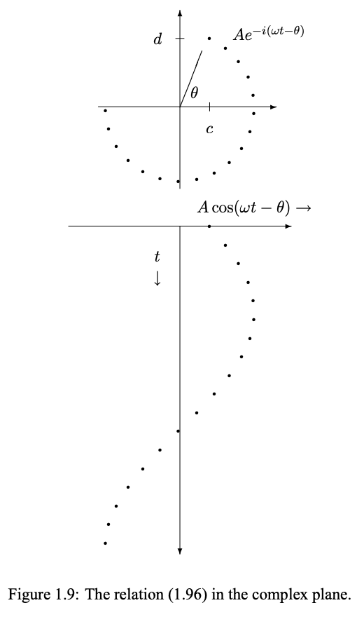
These relations are another example of the equivalence of Cartesian coordinates and polar coordinates, discussed after (1.65). The pair, c and d, are the Cartesian coordinates in the complex plane of the complex number, c + id. The amplitude, A, and phase, θ, are the polar coordinate representation of the same complex (1.96) shows that c and d are also the coefficients of cos ωt and sin ωt in the real part of the product of this complex number with −iωt e . This relation is illustrated in figure 1.9 (note the relation to figure 1.4). As z moves clockwise with constant angular velocity, ω, around the circle, |z| = A, in the complex plane, the real part of z undergoes simple harmonic motion, A cos(ωt − θ). Now that you know about complex numbers and complex exponentials, you should go back to the relation between simple harmonic motion and uniform circular motion illustrated in figure 1.4 and in supplementary program 1-1. The uniform circular motion can interpreted as a motion in the complex plane of the

\[z(t) = e^{-iwt}\]

As t changes, z(t) moves with constant clockwise velocity around the unit circle in the complex plane. This is the clockwise motion shown in program 1-1. The real part, cos ωt, executes simple harmonic motion.

Note that we could have just as easily taken our complex solution to be \(e^{+iwt}\). This would correspond to counterclockwise motion in the complex plane, but the real part, which is all that matters physically, would be unchanged. It is conventional in physics to go to complex solutions proportional to \(e^{−iωt}\). This is purely a convention. There is no physics in it. However, it is sufficiently universal in the physics literature that we will try to do it consistently here.