6.3: Chapter Checklist

Learning Objectives

You should now be able to:

1. Take the limit of a space translation invariant discrete system as the distance between the parts goes to zero, interpret the physics of the resulting continuous system, and find its dispersion relation;
2. Use the Fourier series to set up and solve the initial value problem for a massive string with various boundary conditions.

Problems

6.1. Consider the continuous string of (6.7)-(6.10) as the continuum limit of a beaded string with $W$ beads as $W \rightarrow \infty$. Write the analog of (6.8) and (6.10) for finite $W$. Show that the limit as $W \rightarrow \infty$ yields (6.10). Hint: This is an exercise in the definition of an integral as the limit of a sum. But to do the first part, you will either need to use normal coordinates, X or prove the identity

$$\begin{aligned} \sum_{k=1}^{W} \sin \frac{n k \pi}{W+1} \sin \frac{n^{\prime} k \pi}{W+1} = \begin{cases}b & \text { if } n=n^{\prime} \neq 0 \\ 0 & \text { if } n \neq n^{\prime} \text { and } n, n^{\prime}>0\end{cases} \end{aligned}$$

for a constant $b$ and find $b$.

6.2. Do the integrals in (6.20). Hint: Use integration by parts and watch for miraculous cancellations.

6.3. Find the normal modes of the string with two free ends, shown in Figure $6.7$.

6.4. Fun with Fourier Series and Fractals

In this problem you will explore the Fourier series for an interesting set of functions. Consider a function of the following form, defined on the interval [0,1]: $$f(t)=\sum_{j=0}^{\infty} h^{j} g\left(\operatorname{frac}\left(2^{j} t\right)\right) .$$

Figure $6.7$: A continuous string with both ends free to oscillate in the transverse direction.

where $$g(t)=\left\{\begin{array}{c} 1 \text { for } 0 \leq t \leq w \\ 0 \text { for } w<t<1-w \\ 1 \text { for } 1-w \leq t \leq 1 \end{array}\right.$$

and $\operatorname{frac}(x)$ denotes the fractional part, i.e. $\operatorname{frac}(4.39)=0.39$. $f(t)$ thus depends on the two parameters $h$ and $w$, where $0 < h < 1$ and $0 < w < 1 / 2$. For example, for $h = 1 / 2$ and $w = 1 / 4$, the $h^{0}$ term is shown in Figure \( 6.8.

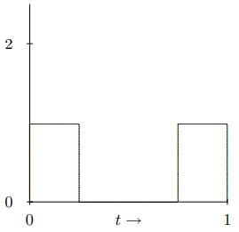
Figure $6.8$: The $h^{0}$ term in $f(t)$ for $h = 1 / 2$ and $w = 1 / 4$.

If we add in the $h^{1}$ term we get the picture in Figure $6.9$.

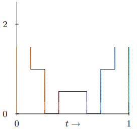
Figure $6.9$: The first two terms in $f(t)$ for $h = 1 / 2$ and $w = 1 / 4$.

Adding the $h^{2}$ term gives the picture in Figure $6.10$, and so on.

The final result is a very bumpy function, called a “fractal.” You cannot compute this function exactly, but you can include enough terms to get to any desired accuracy. Because

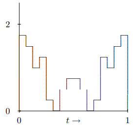
Figure $6.10$: The first three terms in $(f(t)$ for $h = 1 / 2$ and $w = 1 / 4$.

the function is symmetric about $t = 1 / 2$, it is really only necessary to plot it from $0$ to $1 / 2$. Also because of the symmetry, it can be expressed in terms of a Fourier series of cosines, $$f(t)=\sum_{k=0}^{\infty} b_{k} \cos 2 \pi k t .$$

Show that the Fourier coefficients are given by $$b_{k}=\frac{2}{\pi k} \sum_{j=0}^{\xi(k)}(2 h)^{j} \sin \left(2 \pi k w / 2^{j}\right)$$

for $k \neq 0$, and $$b_{0}=\frac{2 w}{1-h}$$

where the function, $\xi(k)$ is the number of times 2 appears as a factor of $k$. Thus $\xi(0)=\xi(1)=\xi(3)=0, \xi(2)=1, \xi(4)=2,$ etc.

Write a program to display and print the fractal for some set of parameters, $h$ and $w$. Also, display the truncated Fourier series, $$f_{m}(t)=\sum_{k=0}^{m-1} b_{k} \cos 2 \pi k t$$

with m terms, for $m = 5$, $10$, and $20$ (or more if you have a fast computer).