11.9: Chapter Checklist

You should now be able to:

1. Interpret plane waves in two- and three-dimensional space in terms of a \(\vec{k}\) vector, angular wave number;
2. Analyze the scattering of a plane wave from a plane boundary between regions with different dispersion relations;
3. Derive and use Snell’s law;
4. Understand the phenomenon of total internal reflection, along with the general statement of the boundary condition at infinity for complex \(\vec{k}\);
5. Understand the physics and mathematics of tunneling phenomena;
6. Understand how degeneracy of the frequencies of the normal modes affects the forced oscillation problem and find the sand patterns on square Chladni plates;
7. Understand the propagation of waves in waveguides, using separation of variables to construct the modes and interpret the result in terms of zig-zag waves;
8. Be able to analyze water waves, ignoring viscosity and angular momentum.
9. Solve problems involving spherical waves where the displacement involves only \(r\) and \(t\);

Problems

11.1. Consider the free transverse oscillations of the two-dimensional beaded string shown in Figure \( 11.59\). All the horizontal strings have tension \(T_{h}\), all the vertical strings have tension \(T_{v}\), all the solid circles are beads with mass \(m\). The square frame is fixed in the \(z = 0\) plane.

1. Find the normal modes and their corresponding frequencies.
2. Suppose that \(T_{v}=100 T_{h}\). Draw nine diagrams, one for each normal mode, in order of increasing frequency indicating which beads are moving up (by a + sign), which are moving down (by a − sign), and which are not moving (by a 0). You can interchange + and − and still have the right answer by changing the setting of your clock, or multiplying your normal mode vector by −1. For example, the lowest frequency mode looks like

while the mode with the fifth highest (and also the fifth lowest — in other words the one in the middle) looks like

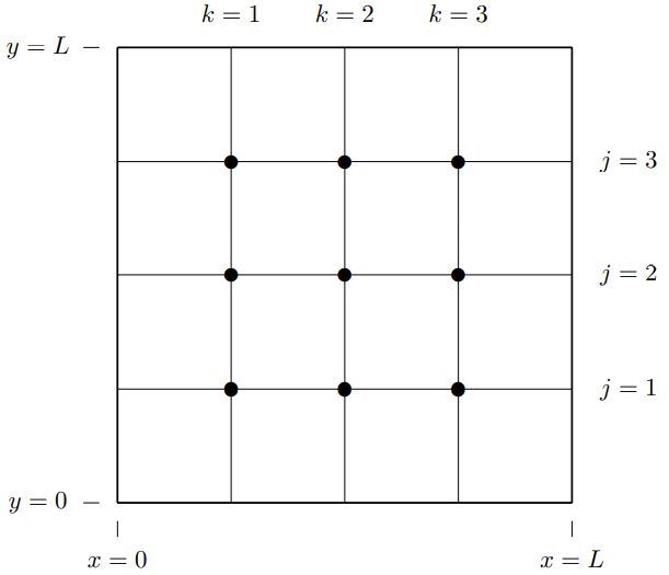
Figure \( 11.59\): A two-dimensional beaded string.

Do the rest and get the order right. You should be able to do this even if you got confused by the details of part a.

11.2. Consider the forced transverse oscillations of the two-dimensional beaded string shown in Figure \( 11.60\). All the strings have tension \(T\), all the solid circles are beads with mass \(m\). The frame is held fixed in the \(z = 0\) plane. The open circles are moved up and down out of the plane of the paper with the same transverse displacement, \[z_{1}(t)=z_{2}(t)=z_{3}(t)=d \cos \omega t\]

where \[\omega=2 \sqrt{\frac{T}{m a}} .\]

Find the displacement for each of the beads. You can do this by solving for the displacement, \(z_{j k}(t)\), of the bead whose horizontal position is \[x=\frac{k L}{4}, \quad y=\frac{j L}{4}\]

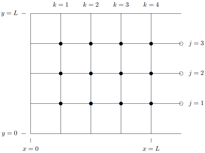
Figure \( 11.60\): A two-dimensional beaded string.

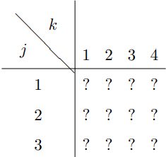
for all relevant \(j\) and \(k\). All displacements will be proportional to \(d \cos \omega t\), so write your answer in the form of a table of the coefficients of \(d \cos \omega t\) for each \(j\) and \(k\):

11.3. Consider the forced transverse oscillations of the semi-infinite two-dimensional beaded string shown in Figure \( 11.61\). All the strings have tension \(T\), all the solid circles are beads with mass \(m\). The equilibrium separations of the blocks are all \(a\). The frame at \(y = 0\) and \(y = 4a\) is held fixed in the \(z = 0\) plane. The open circles at \(x = 0\) are moved up and

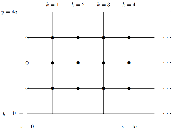
Figure \( 11.61\): A semi-infinite two-dimensional beaded string.

down out of the plane of the paper with transverse displacement, \[z_{1}(t)=z_{3}(t)=\frac{d}{\sqrt{2}} \cos \omega t, \quad z_{2}(t)=-d \cos \omega t ,\]

for the values of \(\omega\) given below. For each \(\omega\) find the displacement for each of the beads as a function of its equilibrium position. That is, determine \(\psi(x, y, t)\). Assume that the entire system is oscillating with frequency \(\omega\) and that the displacement is well-behaved at \(x=+\infty\).

1. Find \(\psi(x, y, t)\) for \[\omega^{2}=\frac{T}{a m}\left(2+\sqrt{2}-\epsilon^{2}\right)\]

In both \(a\) and \(b\), assume that \(\epsilon\) is a small real number, small enough so that you can approximate \[\sinh \frac{\epsilon}{2} \approx \frac{\epsilon}{2} .\]

2. Find \(\psi(x, y, t)\) for \[\omega^{2}=\frac{T}{a m}\left(6+\sqrt{2}+\epsilon^{2}\right) .\]

11.4. A flexible membrane with surface tension \(\tau_{S}\) and surface mass density \(\rho_{S}\) is stretched so that its equilibrium position is the \(z = 0\) plane. Attached to the surface of the membrane at \(x = 0\) is a string with tension \(\tau_{L}\) and linear mass density \(\rho_{L}\). Consider a traveling wave on the membrane with transverse displacement \[\psi(x, y, t)=\psi_{-}(x, y, t)=A e^{-i \omega t+i k_{x} x+i k_{y} y}+R A e^{-i \omega t-i k_{x} x+i k_{y} y}\]

for \(x \leq 0\), and \[\psi(x, y, t)=\psi_{+}(x, y, t)=T A e^{-i \omega t+i k_{x} x+i k_{y} y}\]

for \(x \geq 0\).

In what direction is the reflected wave (for \(x < 0\)) traveling? Easy!

Newton’s law for a small element of the string of length \(d_{y}\) with equilibrium position \((0, y, 0)\) is \[\begin{gathered}
\tau_{S} d y\left[\frac{\partial}{\partial x} \psi_{+}(0, y, t)-\frac{\partial}{\partial x} \psi_{-}(0, y, t)\right]+\tau_{L} d y \frac{\partial^{2}}{\partial y^{2}} \psi_{\pm}(0, y, t) \\
=\rho_{L} d y \frac{\partial^{2}}{\partial t^{2}} \psi_{\pm}(0, y, t) .
\end{gathered} \]

Explain the physical significance of the term above, proportional to \(\tau_{S}\). What is pulling on what? Why does it have the form shown above?

11.5. Consider the transverse oscillations of an infinite flexible membrane stretched in the \(z = 0\) plane with surface tension \(T_{s}\) and surface mass density \(D_{s}\). Along the \(z = 0\), \(x = 0\) line, a string with linear mass density \(D_{L}\) but no tension of its own is attached to the membrane.

Consider a wave of the form: \[\begin{array}{cl}
A e^{i(k x \cos \theta+k y \sin \theta-\omega t)}+R A e^{i(-k x \cos \theta+k y \sin \theta-\omega t)} & \text { for } x<0 \\
T A e^{i\left(k^{\prime} x \cos \theta^{\prime}+k^{\prime} y \sin \theta^{\prime}-\omega t\right)} & \text { for } x>0
\end{array}\]

where \(\cos \theta>0\) and \(\cos \theta^{\prime}>0\).

Find \(\sin \theta^{\prime}\) in terms of \(\sin \theta\) (TRIVIAL!).

Find \(R\) and \(T\).

Hint: Consider \(F = ma\) for an infinitesimal piece of the weighted string, remembering that it has no tension of its own.

11.6. Two semi-infinite flexible membranes are stretched in the \(z = 0\) plane. The first has surface tension \(1 \text { dyne/cm }\) and mass density \(169 \mathrm{gr} / \mathrm{cm}^{2}\). It is fixed along the \(z = 0\), \(y = 0\) axis and the \(z = 0\), \(y = a\) axis and extends from \(x = 0\) to \(\infty\) in the \(+ x\) direction. The second has the same surface tension but mass density \(180 \mathrm{gr} / \mathrm{cm}^{2}\). It is also fixed along the \(z = 0\), \(y = 0\) axis and the \(z = 0\), \(y = a\) axis and extends from \(x = 0\) to \(- \infty\) in the \(− x\) direction. The two membranes are joined together with massless tape at \(x = 0\). Consider the transverse oscillations of this system of the following form: \[\begin{aligned}
\psi(x, y, t)=A \sin \left(k_{y} y\right)\left(e^{-i\left(\omega t-k_{x} x\right)}+R e^{-i\left(\omega t+k_{x} x\right)}\right) & & \text { for } x \leq 0 \\
\psi(x, y, t)=A \sin \left(k_{y} y\right) T e^{-i\left(\omega t-k_{x}^{\prime} x\right)} & & \text { for } x \geq 0
\end{aligned}\]

where \(k_{y}=12 \pi \mathrm{cm}^{-1}\) and \(\omega=\pi \mathrm{s}^{-1}\).

Find \(k_{x}\) and \(\text { [ }\).

Find \(R\) and \(T\).

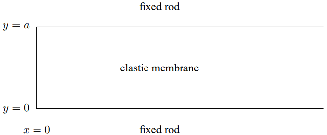
Figure \( 11.62\): A forced oscillation problem in an elastic membrane.

11.7. A uniform membrane is stretched in the \(z = 0\) plane, as shown in Figure \( 11.62\). It is attached to fixed rods along \(y = 0\), \(z = 0\) and \(y = a\), \(z = 0\) from \(x = 0\) to \(\infty\). \(\psi(x, y, t)\) is the \(z\) displacement of the point on the membrane with equilibrium position \((x, y, 0)\). For small oscillations, \(\psi\) satisfies the two-dimensional wave equation, \[v^{2}\left(\frac{\partial^{2}}{\partial x^{2}}+\frac{\partial^{2}}{\partial y^{2}}\right) \psi=\frac{\partial^{2}}{\partial t^{2}} \psi .\]

If this system is extended to an infinite system by continuing it to negative \(x\), show that the normal modes of the infinite system take the form: \[\psi(x, y)=A \sin \left(n k_{0} y\right) e^{i k x} . .\]

Find \(k_{0}\). Suppose that the end of the membrane at \(x = 0\) is driven as follows: \[\psi(0, y, t)=\cos \left(5 v k_{0} t\right)\left[B \sin \left(3 k_{0} y\right)+C \sin \left(13 k_{0} y\right)\right]\]

The boundary condition at \(\infty\) is such that there is no wave traveling in the \(− x\) direction along the membrane. Find \(\psi(x, y, t)\).

Explain the following statement: For \(\omega<2 v k_{0}\), the system acts like a one-dimensional wave carrier with the dispersion relation \(\omega^{2}=v^{2} k^{2}+\omega_{0}^{2}\). What is \(\omega_{0}\)?

11.8. Consider a rigid spherical shell of inner radius \(L\) filled with gas in which the speed of sound is \(v\). In this sphere there are standing wave normal modes of many kinds. We will be interested in those in which the pressure depends only on the distance, \(r\), from the center of the sphere. Suppose that \(\psi(\vec{r}, t)=\chi(r, t)\) is the difference between the pressure of the gas in such a mode and the equilibrium pressure. We know from (11.173) that \(\xi(r, t) \equiv r \chi(r, t)\) satisfies the one-dimensional wave equation: \[\frac{\partial^{2}}{\partial t^{2}} \xi(r, t)=v^{2} \frac{\partial^{2}}{\partial r^{2}} \xi(r, t) .\]

Explain the physics of the boundary condition at \(r = 0\).

In terms of an unknown wave number, \(k\), find a form for \(\chi(r, t)\) that satisfies the boundary condition at \(r = 0\).

Explain the physics of the boundary condition at \(r = L\).

Write down the mathematical statement of the boundary condition at \(r = L\), the solutions of which give the allowed values of \(k\) for the normal modes.

Hints:. Remember that it is \(\chi\) and not \(\xi\) that is the physical pressure difference. The lowest nontrivial mode has a \(k\) value which satisfies \(k L \approx 4.4934\). The amplitude of the pressure oscillations in this mode as a function of \(r\) is shown in the graph in Figure \( 11.63\).

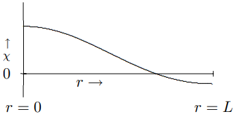
Figure \( 11.63\): Amplitude of pressure oscillation versus \(r\).

11.9. Consider a boundary between two semi-infinite membranes stretched in the \(x\)-\(y\) plane. The membrane for \(x < 0\) has surface tension \(\tau_{s}\) and surface mass density \(\rho_{s}\). The membrane for \(x > 0\) has the same surface tension \(\tau_{s}\) but a different surface mass density \(\rho_{s}^{\prime}\). Along the boundary there is a device (I don’t know exactly how it works) that produces a vertical frictional force, proportional to minus the vertical velocity of the membrane at the boundary. In other words, if \(\psi(x, y, t)\) is the \(z\) displacement of the membrane as a function of \((x, y)\), then the force (in the \(z\) direction) on a small chunk of the boundary stretching from the point \((0, y)\) to \((0, y + dy)\) is \[d F=-d y \gamma \frac{\partial}{\partial t} \psi(0, y, t) .\]

On the membrane there is a plane wave of the form shown below, with displacement: \[\psi(x, y, t)=A e^{i(k x \cos \theta+k y \sin \theta-\omega t)}\]

for \(x < 0\), and \[\psi(x, y, t)=A e^{i\left(k^{\prime} x \cos \theta^{\prime}+k^{\prime} y \sin \theta^{\prime}-\omega t\right)}\]

for \(x > 0\). The setup is shown in Figure \( 11.64\). The dispersion relation for \(x < 0\) is \[\omega^{2}=\frac{\tau_{s}}{\rho_{s}} \vec{k}^{2}\]

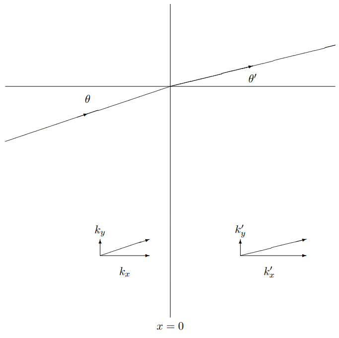
Figure \( 11.64\): Scattering from a boundary in an elastic membrane.

Find \(k^{\prime}\).

Find \(\theta^{\prime}\).

Find \(\gamma\). You should find \(\gamma \rightarrow 0\) for \(\rho_{s} \rightarrow \rho_{s}^{\prime}\). Explain why.

11.10 11-4. Instead of an open ocean, consider a system with a bottom at \(y = 0\) and a fixed top at \(y = 2L\), half full of water and half full of paint-thinner, another nearly incompressible fluid which is lighter than water and floats in the top half without mixing with the water.

Show that waves in this system have the form of (11.122) for \(y \leq L\) (in the water) and \[\begin{gathered}
\psi_{x}(x, y, t)=\mp i e^{\pm i k x-i \omega t} \cosh [k(2 L-y)] , \\
\psi_{y}(x, y, t)=e^{\pm i k x-i \omega t} \sinh [k(2 L-y)] ,
\end{gathered}\]

for \(L \leq y \leq 2 L\) (in the paint-thinner), by arguing that (11.175) and (11.122) satisfy the appropriate boundary conditions at \(y = 0\) and \(y = 2L\) and (for small displacements) at \(y = L\), and show that (11.175), like (11.125), is consistent with incompressibility (\(\vec{\nabla} \cdot \vec{\psi}=0\)).

Show that \(\psi_{x}\) is discontinuous at \(y = L\) and explain physically what is happening at this boundary and why. When you have done this, take a look at program 11-4, in which this system is animated. If you look carefully, you will notice the effect of the breakdown of linearity for large displacements.

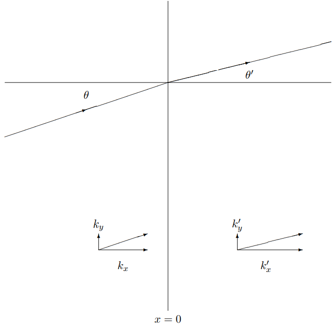
Figure \( 11.64\): Scattering from a boundary in an elastic membrane.

Now suppose that the liquids are contained within vertical walls at \(x = 0\) and \(x = X\).

What boundary conditions are satisfied at the vertical boundaries, \(x = 0\) and \(x = X\)?

Find the form of the displacements for the normal modes in this system. You may want to check that they satisfy \(\vec{\nabla} \cdot \vec{\psi}=0\). Show that the dispersion relation for this system is \[\omega^{2}=\left[\frac{\rho_{W}-\rho_{P}}{\rho_{W}+\rho_{P}} g k+\frac{k^{3} \tau_{S}}{\rho_{W}+\rho_{P}}\right] \tanh k L ,\]

where \(\rho_{P}\) is the density of the paint-thinner, \(\rho_{W}\) is the density of the water, and \(\tau_{S}\) is the surface tension of the boundary between the water and the paint-thinner. Hint: You use an energy argument analogous to (11.127)-(11.137), and just discuss how the various contributions change when you go from (11.137) to (11.176).

11.11. Consider the reflection of sound waves from a massless, infinitely flexible membrane that separates two gases with the same equilibrium pressure, \(p_{0}\), but different densities. The membrane is in the \(x = 0\) plane. The gas in region 1, for \(x < 0\) has equilibrium density \(\rho_{1}\), ratio of specific heat at constant pressure to specific heat at constant volume \(\gamma_{1}\), and sound speed \(\sqrt{\gamma_{1} p_{0} / \rho_{1}}\) while the gas in region 2, for \(x > 0\) has density \(\rho_{2}\), specific heat ratio \(\gamma_{2}\) and sound speed \(\sqrt{\gamma_{2} p_{0} / \rho_{2}}\). A pressure wave in the system has the following form: \[P(r, t) / \delta p=A e^{i \vec{k}_{1} \cdot \vec{r}-i \omega t}+R A e^{i \vec{k}_{R} \cdot \vec{r}-i \omega t}\]

in region 1, for \(x < 0\), and \[P(r, t) / \delta p=T A e^{i \vec{k}_{2} \cdot \vec{r}-i \omega t}\]

in region 2, for \(x > 0\), where \(P(r,t) + p_{0}\) is the pressure of the gas whose equilibrium position is \(\vec{r}\). The small pressure, \(\delta p\), describes the amplitude of the pressure wave. \(R\) and \(T\) are the reflection and transmission coefficients.

The \(k\) vectors are \[\begin{gathered}
\vec{k}_{1}=(k \cos \theta, k \sin \theta, 0) \\
\vec{k}_{R}=\left(-k_{R} \cos \theta_{R}, k_{R} \sin \theta_{R}, 0\right) \\
\vec{k}_{2}=\left(k_{2} \cos \theta_{2}, k_{2} \sin \theta_{2}, 0\right)
\end{gathered}\]

where \(k\), \(k_{R}\), \(k_{2}\), \(\cos \theta\), \(\cos \theta_{R}\), and \(\cos \theta_{2}\) are all positive.

Find \(k_{R}\) and \(\cos \theta_{R}\) in terms of \(k\) and \(\theta\).

Find \(k_{2}\) and \(\cos \theta_{2}\) in terms of \(k\) and \(\theta\).

Show that if \(\rho_{1} / \gamma_{1}>\rho_{2} / \gamma_{2}\), there is a critical value of \(\theta\) above which the wave is totally reflected, and find the critical angle.

To find \(R\) and \(T\), we need the boundary conditions at \(x = 0\). One condition follows from the fact that the membrane is massless and infinitely flexible. That implies that there can be no force on it transverse to its surface.

Find this boundary condition. Hint: Where does the force transverse to the surface come from?

The other condition involves the transverse displacement of the membrane. The displacement can be obtained from the pressure: \[\vec{\psi}(r, t)=\frac{1}{\rho_{j} \omega^{2}} \vec{\nabla} P(r, t) ,\]

where \(\vec{\psi}(r, t)\) is the displacement of the gas whose equilibrium position is \(\vec{r}\) and \(j\) is the region label.

Thus \[\vec{\psi}(r, t) / \delta p=\frac{i A}{\rho_{1} \omega^{2}}\left(\vec{k}_{1} e^{i \vec{k}_{1} \cdot \vec{r}-i \omega t}+R \vec{k}_{R} e^{i \vec{k}_{R} \cdot \vec{r}-i \omega t}\right)\]

in region 1, for \(x < 0\), and \[\vec{\psi}(r, t) / \delta p=\frac{i A}{\rho_{2} \omega^{2}} T \vec{k}_{2} e^{i \vec{k}_{2} \cdot \vec{r}-i \omega t}\]

in region 2, for \(x > 0\).

Find the other boundary condition. Hint: Assume that the amplitude \(\delta p\) is small.

Find \(R\) and \(T\).

11.12. Consider a universe filled with material that has a nonzero conductivity, \(\sigma\). That is, in this material, there is a current proportional to the electric field (Ohm’s law), \[\vec{J}(\vec{r}, t)=\sigma \vec{E}(\vec{r}, t) .\]

We will assume that the material has no other electrical properties, in particular that there is no polarization or magnetization, and that no charge builds up anywhere, so that \(\rho = 0\). Consider the propagation of a plane electromagnetic wave in this universe. Because this universe is perfectly space translation invariant and rotation invariant, and because (11.177) is linear, we would expect that there will be plane wave solutions in which the electric and magnetic fields are proportional to \[e^{i(\vec{k} \cdot \vec{r}-\omega t)}\]

for \(\vec{k}^{2}\) and \(\omega\) related by some dispersion relation. In particular, consider propagation in the \(+z\) direction with the electric field in the \(x\) direction and the magnetic field in the y directions: \[\begin{array}{ll}
E_{x}(\vec{r}, t)=E e^{i(k z-\omega t)}, & E_{y}(\vec{r}, t)=E_{z}(\vec{r}, t)=0 . \\
B_{y}(\vec{r}, t)=B e^{i(k z-\omega t)}, & B_{x}(\vec{r}, t)=B_{z}(\vec{r}, t)=0 .
\end{array}

1. Show from the relevant Maxwell’s equations, \[\begin{gathered}
   \frac{\partial}{\partial z} E_{x}-\frac{\partial}{\partial x} E_{z}=-\frac{\partial B_{y}}{\partial t} \\
   \frac{\partial}{\partial y} B_{z}-\frac{\partial}{\partial z} B_{y}=\mu_{0} \epsilon_{0} \frac{\partial E_{x}}{\partial t}+\mu_{0} J_{x}
   \end{gathered}\]
   that such a plane wave can exist if \[k^{2}=\mu_{0} \epsilon_{0} \omega^{2}+i \mu_{0} \sigma \omega .\]

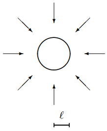
Figure \( 11.65\): A spherical sound damper.

2. Assume that \(\omega\) is real and positive and that the real part of \(k\) is positive. Find the sign of the imaginary part of \(k\), and interpret your result physically. That is, explain why the sign had to come out the way it did.

11.13. Consider a spherical sound wave coming in from far away and being completely absorbed by a spherical sound damper at a radius \(r = \ell\), as shown in Figure \( 11.65\). The pressure in is this system is described by the real part of the complex traveling wave below, depending only on the radius and time: \[p(r, t)-p_{0}=\frac{\epsilon}{r} e^{-i(k r+\omega t)}\]

where \[\omega^{2}=\frac{\gamma p_{0}}{\rho} \vec{k}^{2}\]

with \(p_{0}\), the equilibrium pressure and \(\rho\) the equilibrium mass density of the gas. The typical displacement of the air from its equilibrium position in this wave is in the radial direction, \[\psi_{r}(r, t)=\frac{1}{\rho \omega^{2}} \frac{\partial p}{\partial r} .\]

1. Find the time-averaged power absorbed by the spherical damper at \(r = \ell\).
2. Explain (qualitatively) the factor of \(1 / r\) in the pressure.

Now suppose that there is a massless, flexible spherical boundary between two different gases at radius \(r = r_{b}\), shown as the dashed circle in the diagram in Figure \( 11.66\). The equilibrium pressure, \(p_{0}\), is the same on both sides of the boundary. Also, assume that \(\gamma\) is

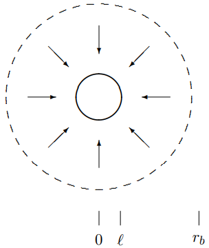
Figure \( 11.66\): A spherical sound damper with a reflecting boundary.

the same for both gases and that the only difference is the densities. Inside the density is \(\rho\), and outside the density is \(\rho^{\prime}\). Now for \(\ell<r<r_{b}\), the pressure is still given as above, but in the region outside the dashed circle, there is a reflected wave as well as the incoming wave, \[p(r, t)-p_{0}=\frac{A}{r} e^{-i\left(k^{\prime} r+\omega t\right)}+\frac{B}{r} e^{i\left(k^{\prime} r-\omega t\right)}\]

where \[\omega^{2}=\frac{\gamma p_{0}}{\rho^{\prime}} \overrightarrow{k^{\prime}}^{2} .\]

3. What are the boundary conditions at \(r = r_{b}\) and why?
4. Find \(B / A\) and \(\epsilon / A\) in the limit, \[k, k^{\prime} \gg \frac{1}{r_{b}}\]

in which you can drop terms proportional to \(1 / r_{b}\) compared to \(k\) or \(k^{\prime}\).

11.14. One of the problems with glass lenses is that the index of refraction of glass depends on frequency. Thus, according to the lens maker’s formula, the focal length of a glass lens will depend of frequency, and that is not good, because if one color is focused sharply, the others will be fuzzy. This is called “chromatic aberration.” Fortunately, different kinds of glass have different behavior in this respect, and this makes it possible to eliminate chromatic aberration. Suppose that you make a lens that looks like this by gluing together lenses made of two different types of glass.

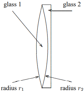
Suppose that the indices of refraction of the two glasses are \[n_{1}(\lambda)=n_{1}^{0}+\alpha_{1} \lambda, \quad n_{2}(\lambda)=n_{2}^{0}+\alpha_{2} \lambda .\]

What relation must be satisfied if the compound lens is to have a focal length that is independent of \(\lambda\)?

11.15. You can also make a telescope with one converging lens (the objective) and one diverging lens (the eyepiece).

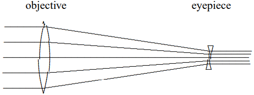
The focal length of the convex lens is \(f_{1}\) and the focal length of the concave lens is \(-f_{2}\).

1. If the ray tracing works as shown, that is that parallel rays entering the objective are focused down to parallel rays leaving the eyepiece, find the distance, \(d\), between the two lenses.
2. Compute the magnification by assuming that you are looking at a distance object which subtends an angular size \(\theta\). Then consider a ray at angle \(\angle\) that passes through the center of the convex lens. By calculating where it passes through the concave lens, you should be able to determine its angle, \(\theta_{o}\), when it reaches the observers eye. The magnification is then \(\theta_{o} / \theta\). What is it in terms of the focal lengths?
3. The image in this case is right-side-up. Draw a careful diagram to explain why.

11.16. The appearance of the rainbows depends dramatically on the index of refraction of water. Describe in detail what the rainbows look like if \(n\) were decreased by 0.03 for each frequency of light? Discuss the first and second rainbows and Alexander’s dark band.